In this complete guide, you’ll learn how to use the Python Optuna library for hyperparameter optimization in machine learning. In this blog post, we’ll dive into the world of Optuna and explore its various features, from basic optimization techniques to advanced pruning strategies, feature selection, and tracking experiment performance.
You’ll also learn how to visualize your optimization results with built-in plots and save your optimization sessions for resuming or sharing across multiple processes. By the end of this guide, you’ll have a solid understanding of how to harness the power of Optuna to fine-tune your machine-learning models and achieve top-notch performance. So, let’s get started and unlock the full potential of your machine-learning projects with Optuna!
Table of Contents
Hyper-Parameters in Machine Learning
Before we dive into tuning your hyper-parameters, let’s take a moment to recap what the differences between parameters and hyper-parameters are in a machine learning model.
Parameters in a machine learning model refer to the variables that an algorithm itself produces (such as a coefficient) to produce a prediction. These parameters are not set or hard-coded and depend on the training data that is passed into your model. Because of this, they’re likely to change when your data changes.
On the other hand, hyper-parameters are variables that you specify while building a machine-learning model. This means that it’s the user that defines the hyper-parameters while building the model. For example, in a k-nearest neighbour algorithm, the hyper-parameters can refer the value for k or the type of distance measurement used.
In short, hyper-parameters control the learning process, while parameters are learned.
This is where the “art” of machine learning comes into play. The choice of your hyper-parameters will have a significant impact on the success of your model. Being able to tune your model is finding what the best hyper-parameters are.
Hyper-Parameter Tuning in Machine Learning
Hyper-parameter tuning refers to the process of find hyper-parameters that yield the best result. This, of course, sounds a lot easier than it actually is. Finding the best hyper-parameters can be an elusive art, especially given that it depends largely on your training and testing data.
One way to tune your hyper-parameters is to use a grid search. This is probably the simplest method as well as the crudest. In a grid search, you try a grid of hyper-parameters and evaluate the performance of each combination of hyper-parameters.
An alternative to this is to use Optuna! Let’s dive into how this works.
Understanding the Need for Optuna
Optuna is a hyperparameter tuning library that is specifically designed to be framework agnostic. This means that you can use it with any machine learning or deep learning framework.
Optuna offers three distinct features that make it an optimal hyperparameter optimization framework:
- Eager search spaces: automated search for optimal hyperparameters
- State-of-the-art algorithms: efficiently search large spaces and prune uncompromising trials for faster results
- Easy parallelization: parallelize hyperparameter search over multiple threads or processes without modifying code
Throughout this guide, we’ll start by using Optuna with sklearn since it’s a very approachable machine learning framework.
Getting Started with Optuna
In this section, we’ll dive into how to get started with Optuna. We’ll start by covering how to install Optuna, what a basic optimization script looks like, and how to run a small optimization process. Let’s get started!
Installing Optuna in Python
In order to install Optuna, we can use the pip package manager. To do this, we can use the following command:
pip install optunaRunning this command in your terminal will install the package. After that, you can import the library using the import command:
import optunaFollowing this, we’re ready to dive into creating the basic structure of an Optuna optimization script.
Basic Structure of an Optuna Optimization Script
Before we dive into creating an optimization script, let’s first take a look at the structure of what this looks like. The overall process works differently from the brute-force approach of GridSearchCV . Because of this, let’s cover off the different components of the process:
- Defining the Objective Function
- Creating a Study Object
- Running the Optimization Process
The objective function is at the core of how Optuna optimizes the hyperparameter selections. While a brute-force grid search also seeks to minimize an objective function, it doesn’t actually take into account what combination of hyperparameters is doing well or not.
Let’s take a look at what this overall process looks like:
# Understanding the Optuna Optimization Process
import optuna

# 1. Define the Objective Function
def objective(trial):
    # Define hyperparameters and model
    # Train and evaluate the model
    # Return the evaluation metric

# 2. Create a Study Object
study = optuna.create_study(direction='maximize')

# 3. Run the Optimization Process
study.optimize(objective, n_trials=100)
We can see how simple the process appears to be. However, there’s quite a bit happening under the hood. For example, the objective function we develop is actually creating and fitting our model. Similarly, it creates predictions and scores them against the evaluation metric, which the function returns.
By creating a study, we instruct Optuna to either aim to maximize or minimize one or more evaluation metrics. In the final step, we run the study by calling the .optimize() method, which takes the object function and the number of trials to run as parameters.
An Example of Using Optuna to Optimize Hyperparameters
Now that you have a good understanding of how Optuna is used to optimize hyperparameters, let’s walk through an example of how this works in practice.
We’ll use a simple sklearn example to illustrate how the process works. While Optuna works with more complex models (and frameworks), we’ll keep things simple to make sure it’s easy to follow.
For this example, we’ll use the iris dataset to classify flowers using a support vector machine model:
# Loading our datasets
from sklearn.datasets import load_iris
from sklearn.model_selection import train_test_split

iris = load_iris()
X_train, X_test, y_train, y_test = train_test_split(
	iris.data,
	iris.target,
	test_size=0.2,
	random_state=42
)
In the code block above, we imported the iris dataset. We then split the dataset into a training and testing datasets using the train_test_split() function.
Creating an Objective Function for Optuna
Let’s now dive into how we can create an objective function to prepare for our Optuna study! The objective function should return one or more criteria that evaluate a model’s performance. Let’s take a look at how we can create an objective function:
# Creating an Objective Function
from sklearn.svm import SVC
from sklearn.metrics import accuracy_score

def objective(trial):
    # Define hyperparameters
    c = trial.suggest_float("C", 1e-10, 1e10, log=True)
    kernel = trial.suggest_categorical("kernel", ["linear", "poly", "rbf", "sigmoid"])

    # Create and train the model
    svm = SVC(C=c, kernel=kernel, random_state=42)
    svm.fit(X_train, y_train)

    # Evaluate the model
    y_pred = svm.predict(X_test)
    accuracy = accuracy_score(y_test, y_pred)

    return accuracy
Notice in the code block above that we’re only creating an objective function. The function takes a single argument: the trial. We’re then using this trial inside of our function to suggest some hyperparameter values.
Rather than specifying unique values to test for, we’re creating our search space based on suggestions. In particular, we’re using two methods here: .suggest_float() and .suggest_categorical() to define our search space for the two hyperparameters C and kernel. We won’t go into the mechanics behind support vector machines here, but they can be used for both classification and regression tasks.
We’ll dive into the other methods available later in the tutorial. For now, let’s discuss what they do in principle. The .suggest_categorical() method in our example above has two parameters: name which represents the name of the hyperparameter and choices, which represents the different candidates available.
Running the Optuna Optimization Process
With the objective function defined, we can now create a study object. This object allows us to run the optimization process. The study object is created using the create_study() function, which defines the direction (or directions) that we want to optimize our criteria by.
The create_study() function takes a parameter, direction=, which allows us to specify the direction in which we want the evaluation criteria should go in.
In our example, we return the accuracy of our model. We want the accuracy of our model to increase, meaning that we should pass in we want the data to 'maximize' the direction. To learn more about how to use metrics such as accuracy to evaluate machine learning models, check out this guide on using a confusion matrix to evaluate performance.
Let’s see what this looks like:
# Creating and running our optimization
import optuna
study = optuna.create_study(direction='maximize')
study.optimize(objective, n_trials=100)
In our example, we instruct Optuna to run 100 trials by specifying that we want the evaluation criteria to increase.
After the optimization process is complete, you can access the best trial and its hyperparameters using the best_trial and best_params attributes of the study object:
# Evaluating our Optuna Trial
print("Best trial:", study.best_trial.number)
print("Best accuracy:", study.best_trial.value)
print("Best hyperparameters:", study.best_params)

# Returns:
# Best trial: 0
# Best accuracy: 1.0
# Best hyperparameters: {'C': 48.67813691808164, 'kernel': 'linear'}
We can see from the code block above that the study object maintains a lot of information about the different trials. We can access this information by using different attributes, such as the ones listed above.
For example, by using the .best_params attribute, we can see which of the different hyperparameters returned the optimal results.
Understanding Optuna’s Search Distributions
Optuna defines the search spaces by defining the range and type of values that can be explored during the hyperparameter optimization process. We can define the search space by specifying the distributions for each hyperparameter, where different samplers are used to sample values from the distributions.
Optuna suggest_categorical
suggest_categorical(param_name, choices): This method suggests a categorical parameter, which can take one of the given choices. The choices are a list of possible values for the parameter. Optuna will explore different combinations of these choices to find the best hyperparameters.
Optuna suggest_int
suggest_int(param_name, low, high, step=1, log=False): This method suggests an integer parameter within the specified range [low, high]. You can also define the step size and whether to use logarithmic scaling.
Optuna suggest_float
suggest_float(param_name, low, high, step=None, log=False): This method suggests a floating-point parameter within the specified range [low, high]. You can also define the step size and whether to use logarithmic scaling.
Optuna suggest_loguniform
suggest_loguniform(param_name, low, high): This method suggests a floating-point parameter from a log-uniform distribution within the specified range [low, high]. It’s useful for parameters that have a multiplicative effect, such as learning rates and regularization coefficients.
Optuna suggest_discrete_uniform
suggest_discrete_uniform(param_name, low, high, q): This method suggests a floating-point parameter from a discrete uniform distribution within the specified range [low, high], with a step size of ‘q’. It’s useful for parameters that need to be explored with a fixed interval.
Optuna suggest_uniform
suggest_uniform(param_name, low, high): This method suggests a floating-point parameter from a uniform distribution within the specified range [low, high]. It’s useful for parameters that have an additive effect, such as biases and thresholds.
Understanding Optuna Search Samplers
Optuna also offers a number of different ways to sample hyperparameters from the defined search space. Rather than using the brute-force grid search approach, Optuna allows you to optimize the method by which hyperparameters are selected.
Let’s break down how the different search samplers that the Optuna library offers:
- Tree-structured Parzen Estimator (TPE) Sampler (
TPESampler): This is the default sampler that Optuna uses. The TPE sampler is a Bayesian optimization technique that models the search space by using two estimators: one for the best-performing trials and one for the other trials. - Random Sampler (
RandomSampler): the random sampler is used to sample hyperparameters randomly. This doesn’t take into account the performance of previous trials. The random sampler is a good tool to use for baseline comparisons to evaluate other samplers. - GridSampler (
GridSampler): the GridSampler is used to search across all different hyperparameters in the space. This is very useful when you’re working through a small space of options. - CMA-ES based algorithm (
CmaEsSampler): The Covariance Matrix Adaptation Evolution Strategy (CMA-ES) is a powerful optimization algorithm for continuous search spaces. This type of space works best for continuous search spaces and less well for discrete or categorical hyperparameters. - Partial Fixed Sampler (
PartialFixedSampler): This sampler allows you to fix the values of some hyperparameters while optimizing the others. It can be useful when you want to explore the effect of certain hyperparameters while keeping others constant. - Nondominated Sorting Genetic Algorithm II (
NSGAIISampler): The Nondominated Sorting Genetic Algorithm II (NSGA-II) is a popular multi-objective optimization algorithm. Optuna’sNSGAIISamplerimplements the NSGA-II algorithm for hyperparameter optimization, which can be useful when optimizing multiple objectives simultaneously. - Quasi Monte Carlo Sampling algorithm (
QMCSampler): The Quasi Monte Carlo (QMC) sampling algorithm is a low-discrepancy sequence sampling technique, which can provide better coverage of the search space than random sampling.
You can implement these samplers using the following code, modifying it for the sample that you want to use:
# Specifying a Sampler in Optuna
import optuna
sampler = optuna.samplers.TPESampler(seed=42)
study = optuna.create_study(sampler=sampler, direction='maximize')
Different samplers will work better for different types of models and spaces of hyperparameters. Understanding when to use which sampler can be a helpful toolset for optimizing your hyperparameters quicker.
Using Optuna Pruners for Early Stopping
Optuna provides a number of different pruners that can be used to stop unpromising trials early. This allows you to save a significant amount of time and resources for hyperparameter optimization, especially compared to grid search.
Pruning is especially useful when you’re working with very large datasets or more complex models that can take a long time to train.
Optuna provides the following pruning algorithms:
- Median pruning algorithm implemented in
MedianPruner - Non-pruning algorithm implemented in
NopPruner - Algorithm to operate pruner with tolerance implemented in
PatientPruner - Algorithm to prune specified percentile of trials implemented in
PercentilePruner - Asynchronous Successive Halving algorithm implemented in
SuccessiveHalvingPruner - Hyperband algorithm implemented in
HyperbandPruner - Threshold pruning algorithm implemented in
ThresholdPruner
In most cases the SuccessiveHalvingPruner and HyperbandPruner outperform most of the other pruners. Similar to most things in machine learning, however, much of this is contextual.
Let’s now take a look at how we can implement pruners in our hyperparameter optimization. In order to implement pruning in the hyperparameter optimization process, you’ll need to report the intermediate results of your trials using the trial.report() method.
By using this method, we’re able to stop an experiment early, allowing us to save time and resources. Let’s take a look at what this looks like:
# Using a Pruner to End Experiments Early
from sklearn.model_selection import cross_val_score
from optuna.pruners import SuccessiveHalvingPruner

def objective(trial):
    c = trial.suggest_float("C", 1e-10, 1e10, log=True)
    kernel = trial.suggest_categorical("kernel", ["linear", "poly", "rbf", "sigmoid"])

    svm = SVC(C=c, kernel=kernel, random_state=42)

    for step in range(5):
        score = cross_val_score(svm, X_train, y_train, cv=5, scoring='accuracy').mean()
        trial.report(score, step)

        # Check for pruning
        if trial.should_prune():
            raise optuna.TrialPruned()

    return score

pruner = SuccessiveHalvingPruner(min_resource=1, reduction_factor=2, min_early_stopping_rate=0)
study = optuna.create_study(pruner=pruner, direction='maximize')
study.optimize(objective, n_trials=20)
In the example above, we implemented a new objective function. The function now has a for loop to create cross-validation. During the loop, we report both the score and the step, which Optuna then evaluates using the .should_prune() method. If the thresholds aren’t met, then Optuna will end the experiment early.
Optuna Callbacks: Using Custom Actions During Optimization
Optuna allows you to define and use callbacks during the optimization process, meaning that you can define custom actions. Callbacks are functions that are called at the end of each trial. This means that we can do useful actions, such as logging trial results.
Defining a Custom Callback Function for Optuna
Let’s start by defining a simple callback function to see what this behavior is like. We’ll create a function that simply prints the trial number and its value:
# Create a Simple Callback Function
def print_trial_info(study, trial):
    print(f"Trial {trial.number}: Value = {trial.value}")
We can see that the callback takes two parameters:
- The study and
- The trial
We can use this callback function in our study by passing it into the .optimize() method:
# Passing Our Callback Into the Study
def objective(trial):
    c = trial.suggest_float("C", 1e-10, 1e10, log=True)
    kernel = trial.suggest_categorical("kernel", ["linear", "poly", "rbf", "sigmoid"])

    svm = SVC(C=c, kernel=kernel, random_state=42)
    svm.fit(X_train, y_train)

    y_pred = svm.predict(X_test)
    accuracy = accuracy_score(y_test, y_pred)

    return accuracy

study = optuna.create_study(direction='maximize')
study.optimize(objective, n_trials=20, callbacks=[print_trial_info])
We can see that we passed in the callback as a list into the callbacks= parameter. Let’s explore how we can combine multiple callbacks into the same study.
Combining Multiple Callbacks in Optuna
You can also combine multiple callbacks to perform different actions during the optimization process. Here’s an example of how to use two callbacks: one for printing trial information and another for saving the best model:
# Using Multiple Callbacks in Optuna
import pickle

def save_best_model(study, trial):
    if study.best_trial.number == trial.number:
        best_model = SVC(C=trial.params['C'], kernel=trial.params['kernel'], random_state=42)
        best_model.fit(X_train, y_train)
        with open("best_model.pkl", "wb") as f:
            pickle.dump(best_model, f)

study = optuna.create_study(direction='maximize')
study.optimize(objective, n_trials=20, callbacks=[print_trial_info, save_best_model])
In the example above, we created a second callback function that checks if the current trial is the best trial so far. If that’s the case, it serializes the model and saves it to a file.
By utilizing callbacks in Optuna, you can easily monitor the optimization process, log trial results, or perform other custom actions, providing you with greater control and flexibility during hyperparameter optimization.
Saving and Resuming Optimization Sessions with Optuna’s Storage Options
Optuna allows you to work with different storage options, with which you can save and resume optimization sessions. This can be extremely helpful when you’re working on a long-running optimization process (such as those from complex models). Similarly, it can help when you want to analyze the results of a study later on.
By using storage options, you can save the results of a trial, resume an interrupted optimization session, or even share the optimization session across multiple processes or machines.
Let’s explore how we can use SQLite storage to save our study’s results.
Using SQLite Storage to Save and Resume Optuna Sessions
Optuna supports SQLite for local storage, which is useful for saving and resuming single-process optimization sessions. To use SQLite storage, you need to pass the SQLite database URL to the optuna.create_study() method using the storage parameter.
Let’s take a look at how we can use Optuna to create a study using SQLite storage:
# Creating a Sample Database to Save Results To
import optuna

storage_url = "sqlite:///example.db"
study_name = "svm_optimization"

study = optuna.create_study(storage=storage_url, study_name=study_name, direction='maximize', load_if_exists=True)
study.optimize(objective, n_trials=20)
In the code block above, we declared variables for our database and study name. We then passed these into our study when we create it. The study_name parameter is used to uniquely identify the study, and the load_if_exists parameter is set to True to load the existing study if it already exists in the database.
This allows us to resume the study if it’s interrupted or if we want to continue it. We can do this is by using the following code:
# Resuming an Existing Study
study_resume = optuna.create_study(storage=storage_url, study_name=study_name, direction='maximize', load_if_exists=True)
study_resume.optimize(objective, n_trials=20)
Analyzing the Results of a Saved Optuna Study
We can load the saved study in Optuna by using the load_study() function. This allows us to analyze the results of the study or to perform additional optimizations.
Let’s see how we can load a study and analyze its results:
# Loading a Saved Optuna Study
saved_study = optuna.load_study(study_name=study_name, storage=storage_url)
print("Best trial:", saved_study.best_trial.number)
print("Best value:", saved_study.best_trial.value)
print("Best hyperparameters:", saved_study.best_params)

# Returns:
# Best trial: 15
# Best value: 0.9583333333333334
# Best hyperparameters: {'C': 17306.972770120043, 'kernel': 'linear'}
By using the storage options within Optuna, you’re able to save and resume the different optimization sessions. You can also share the sessions across multiple processes or machines. Finally, you can also analyze the results later, giving you greater flexibility and control over how you optimize hyperparameters.
Visualizing Optimization Results with Optuna’s Built-in Plots
Another great tool built into Optuna is the ability to use built-in plotting functions that allow you to visualize the optimization results. This allows you to analyze the trial’s performance, understand the search space, and make better decisions for your machine-learning models.
Under the hood, Optuna uses Plotly for visualizing the results. If you don’t yet have it installed, you can install it using the command below:
pip install plotlyNow that you have Plotly installed, let’s take a look at some of the different things we can visualize with Optuna.
Plotting Optimization History with Optuna
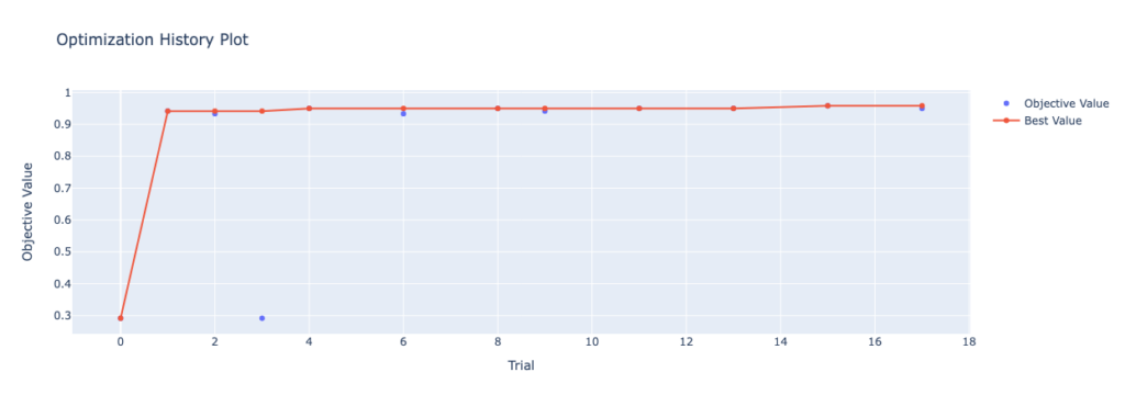
We can use an optimization history plot to visualize the results of our trials over time. This allows you to better understand the optimization process.
In order to plot the optimization history plot, you can use the plot_optimization_history() function. Let’s take a look at how we can do this:
# Plotting Optimization History
import optuna.visualization as vis

optimization_history_plot = vis.plot_optimization_history(study)
optimization_history_plot.show()
By using the code block above, we return the image below. Because we used Plotly to generate the plot, the hovers are interactive and you can zoom into particular sections.
Now, let’s take a look at plotting parameter importance.
Plotting Parameter Importance with Optuna
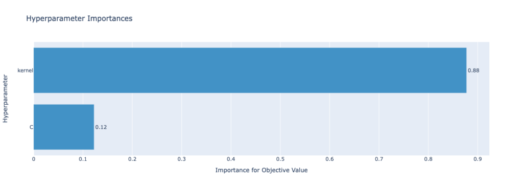
We can also use Optuna to plot parameter importance using the plot_param_importances() function. This allows you to better understand the relative importance of each hyperparameter. This, in turn, allows you to better understand which hyperparameters have more impact on the results of the trial.
Let’s see what this plot looks like for our current study. We can create the plot using the code below:
# Plotting Parameter Importance
param_importance_plot = vis.plot_param_importances(study)
param_importance_plot.show()
This returns the following image:
Let’s now take a look at using contour plots of our optimization study.
Plotting Contour Plots of Optimization with Optuna
The contour plot generated by Optuna will highlight the relationship between two hyperparameters and the trial value. This allows you to better understand the interactions between different hyperparameters. In order to create a contour plot, you can use the plot_contour() function and pass in the study as well as a list of the two hyperparameters you want to analyze.
# Plotting a Contour Plot in Optuna
contour_plot = vis.plot_contour(study, params=["C", "kernel"])
contour_plot.show()
This returns the following image:
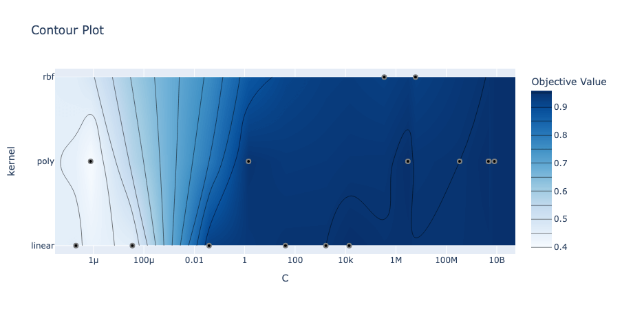
The plot has the two hyperparameters along the x- and y-axes and uses the color of the graph to show the trial value.
Plotting a Slice Plot of Optimization Trials with Optuna
The slice plot shows the relationship between a single hyperparameter and the trial value, which can help you understand the distribution of the trial results for each hyperparameter value. You can create a slice plot using the optuna.plot_slice() function.
Let’s take a look at how to create a slice plot in Optuna:
# Creating a Slice Plot in Optuna
slice_plot = vis.plot_slice(study, params=["C", "kernel"])
slice_plot.show()
Similar to the contour plot, we passed in the study and hyperparameters as a list we wanted to analyze. This returns the following image:
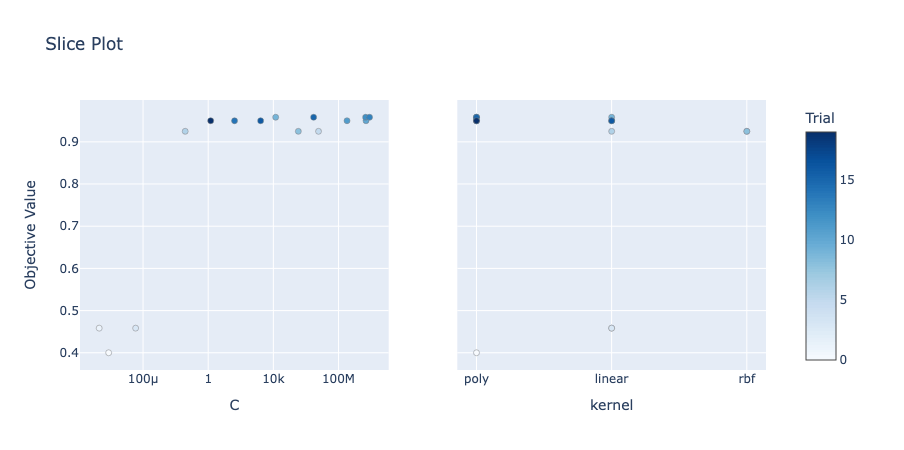
The slice plot allows us to understand different hyperparameters. This allows you to see the values of different hyperparameters and their impact.
Using Optuna for Feature Selection
Optuna goes beyond hyperparameter optimization – it also allows you to better select features. This allows you to improve your machine learning model’s performance and reduce the complexity of your dataset. In this section, we’ll explore how to use Optuna for feature selection.
Feature selection is the process of selecting a subset of relevant features to build a machine-learning model. Optuna can be used to find the optimal combination of features that maximizes model performance. Let’s create an example using the Iris dataset and a RandomForest classifier.
Let’s take a look at what this looks like:
# Feature Selection Using Optuna
import optuna
from sklearn.datasets import load_iris
from sklearn.ensemble import RandomForestClassifier
from sklearn.feature_selection import SelectKBest, f_classif
from sklearn.metrics import accuracy_score
from sklearn.model_selection import train_test_split

# Load the dataset and split it into training and testing sets
iris = load_iris()
X_train, X_test, y_train, y_test = train_test_split(iris.data, iris.target, test_size=0.2, random_state=42)

# Define the objective function
def objective(trial):
    k = trial.suggest_int("k", 1, X_train.shape[1])
    selected_features = SelectKBest(f_classif, k=k).fit_transform(X_train, y_train)

    n_estimators = trial.suggest_int("n_estimators", 10, 100)
    max_depth = trial.suggest_int("max_depth", 2, 10, log=True)

    classifier = RandomForestClassifier(n_estimators=n_estimators, max_depth=max_depth, random_state=42)
    classifier.fit(selected_features, y_train)

    selected_features_test = SelectKBest(f_classif, k=k).fit_transform(X_test, y_test)
    y_pred = classifier.predict(selected_features_test)
    accuracy = accuracy_score(y_test, y_pred)

    return accuracy

study = optuna.create_study(direction='maximize')
study.optimize(objective, n_trials=50)
In this example, we use the SelectKBest function from Sklearn to select the top k features. Notice that we’re using Optuna to help identify the optimal value for k. The function selects features based on their univariate statistical significance using the ANOVA F-value. The objective function optimizes the number of selected features (k) and the hyperparameters of the RandomForest classifier.
Frequently Asked Questions
Optuna is a powerful open-source library in Python designed for hyperparameter optimization in machine learning. It provides an efficient and user-friendly interface for finding the best hyperparameters for machine learning models. Optuna automates the process of selecting optimal hyperparameters through various optimization algorithms, including Tree-structured Parzen Estimator (TPE), and supports advanced features like pruning strategies, feature selection, and experiment tracking.
Yes, Optuna is generally faster and more efficient than GridSearch for hyperparameter optimization. GridSearch is a traditional method that performs an exhaustive search over a specified parameter grid, which can be computationally expensive and time-consuming, especially for large datasets and complex models. In contrast, Optuna uses more advanced optimization algorithms like TPE, which intelligently explores the search space and converges to the optimal solution more quickly. This makes Optuna a better choice for large-scale machine learning projects where time and computational resources are crucial factors.
Optuna is not strictly a Bayesian hyperparameter optimizer, but it does incorporate some Bayesian optimization techniques. Optuna mainly uses the Tree-structured Parzen Estimator (TPE) algorithm, which is a sequential model-based optimization method that shares some similarities with Bayesian optimization. Both methods aim to find the optimal hyperparameters by building a probabilistic model of the objective function and using it to guide the search process. However, TPE is more flexible and efficient than traditional Bayesian optimization, making Optuna a powerful choice for hyperparameter tuning in machine learning.
Conclusion
And there you have it, folks! We’ve successfully navigated through the fascinating world of Optuna and its powerful capabilities for hyperparameter optimization in machine learning. We started off by understanding the basics of Optuna and gradually made our way to more advanced techniques, including pruning strategies, feature selection, and tracking experiment performance.
Along the way, we also discovered how to visualize our optimization results using built-in plots and save our optimization sessions for future resuming or sharing across multiple processes. By now, you should have a strong grasp of how to employ Optuna to fine-tune your machine learning models and achieve outstanding performance.
We hope you found this guide helpful and insightful. Remember, practice makes perfect, so don’t hesitate to apply these techniques to your own machine learning projects and see the improvements firsthand. As always, we’re eager to hear your thoughts, experiences, and any questions you might have. So feel free to drop a comment below and share your Optuna adventures with us!
Keep experimenting, keep learning, and let’s continue to unlock the full potential of our machine learning projects together. Happy optimizing!
To learn more about optuna, check out the official documentation.