The colors of paintings: Blue is the new orange

I made a visualization of the change in colors of paintings over time which a friend tweeted. Several people wanted more info on the method used, so I decided to write a detailed description here, also including the (not very pretty) code I used.

Recently I read a couple of very nice blog post on color use in movies, where colors where extracted from either movie posters or the actual frames of trailers.

I decided to try to do something similar but with data for a longer time period than the era of film. I decided to download images of paintings. So there is a bunch of different sites where you can access (photos of) paintings, e.g. BBC, Google Art Project, Wikiart, Wikimedia commons, and various museums. One of my favorites is the BBC:s site where you can browse through over 200K of well organized paintings! An amazing resource. For many of these there is also information on the year they were painted, the artist, etc.

So let’s use them to visualize the colors in paintings over history!

In order to this, we need first to scrape the images of the paintings from the site, then extract the relevant info from them, and last plot it in a nice way.To do all this I used R.

Scraping

For each of the 4434 pages in the BBC search browser, I saved a file listing the images on that page, the URL to the thumbnails, the year it was painted and some additional info. I did this in a loop and saved each page separately because saving each file takes some time, and I wanted to be able to abort it without losing what I had extracted so far. I then combine all the files into one large file.

library(rvest)
library(pipeR)
 
url="http://www.bbc.co.uk/arts/yourpaintings/paintings/search?=&page="
urls=paste(url, 1:4434, sep="")
 
for (i in 1:length(urls)){
 doc.temp=html(urls[i], encoding="ISO-8859-1")
 files.temp=doc.temp %>>% html_nodes(".thumb") %>>% html_node("img") %>>% html_attr("src")
 links.temp=doc.temp %>>% html_nodes(".thumb") %>>% html_node("a") %>>% html_attr("href")
 doc.temp2=lapply(links.temp, html)
 year=sapply(doc.temp2, function(x) x %>>% html_nodes("#info") %>>% html_nodes("#short-desc") %>>% html_nodes("li") %>% .[[1]] %>>% html_text)
 info=sapply(doc.temp2, function(x) x %>>% html_nodes("#info") %>>% html_nodes("#short-desc") %>>% html_nodes("li") %>% .[[2]] %>>% html_nodes("span") %>% html_text %>% (function(x) {paste(x[1],x[2], sep="")}))
 year=gsub("\t", "", year)
 year=gsub("\r", "", year)
 year=gsub("\n", "", year)
 write.csv(cbind(rep(i, length(files.temp)),links.temp, files.temp, year,info),file=paste("C:/Art/files_bbc/",sprintf("%04d", i), ".csv", sep=""))
 cat("downloaded page", i, "out of", length(urls),"at", as.character(Sys.time()), "\n")
}

files=list.files("C:/Art/files_bbc",full.names=T)
files=lapply(files, function(x) read.csv(x,header=F, skip=1,col.names=c("X","page","link","file","year","info")))
library(plyr)
all=rbind.fill(files)
write.csv(all,file="C:/Art/bbc_df1.csv",row.names=F)

Next I downloaded all the thumbnails from the URLs listed in my file for which there were information on the year they were painted. This was almost 130K images totaling about 2.5 Gb. (Therefor I actually downloaded a few thousands at atime with the sapply command.)

all=read.csv("C:/Art/bbc_df1.csv")
all$file=as.character(all$file)
all=all[grepl("Date painted:",all$year),]
all$year=as.character(all$year)
all$picnr=1:length(all$year)
 
sapply(1:length(all$year), function(x) download.file(url=all$file[x],destfile=paste("C:/Art/data_bbc/",sprintf("%06d", x),sep="", ".jpg"), mode ="wb", quiet = T))

Analyzing

Because the year info is not well formatted some cleaning was needed. A minority of the paintings are ambiguously dated, e.g. “c. 1948”,“1851-1853”, “1803 (?)”, “exhibited 1885“, “possibly 1843”, “1950s”, “early19th century”. I therefore decided to use the first year in all spans and ignore qualifiers like “c.”, “(?)”, “exhibited”, and “possibly”. I decided to exclude vague dates like “1950s” and “early 19th century”.

all$year=as.character(all$year)
all$year[grepl("0s",all$year)]="ambiguous"
all$year=gsub("[[:alpha:]]","", all$year)
all$year=gsub("\\.", "",all$year)
all$year=gsub(":", "",all$year)
all$year=gsub("\\(", "",all$year)
all$year=gsub("\\)", "",all$year)
all$year=gsub("\\?", "",all$year)
## take first year if it's a span
all$year=sapply(strsplit(all$year,"-"), "[", 1)
all$year=sapply(strsplit(all$year,"-"), "[", 1)
all$year=sapply(strsplit(all$year,"–"), "[", 1)
all$year=sapply(strsplit(all$year,"/"), "[", 1)
all$year=sapply(strsplit(all$year,","), "[", 1)
all$year=sapply(strsplit(all$year,"&"), "[", 1)
all$year=sub("^\\s+", "",all$year)
all$year=sapply(strsplit(all$year, ""), "[", 1)
all$year[nchar(all$year)!=4]=NA
all$year=as.numeric(all$year)

I extracted info on what technique was used in the painting, divided into 4 categories: oil, acrylic, tempera, and other/mixed.

all$tech=rep("Other/mixed",length(all$year))
all$tech[grepl("Oil on",all$info)]="Oil"
all$tech[grepl("Acrylic on",all$info)]="Acrylic"
all$tech[grepl("Tempera on",all$info)]="Tempera"

Some of the cataloged paintings on the BBC website lack a proper image. For these the “painting_missing.gif” is used on the website,which means these needs to be excluded (I could have done this already before downloading all the images, but I didn’t realize it until later). Also, a few images are just in a strange format or something went wrong when I downloaded them. These I had to exclude manually.

picnames=sapply(strsplit(as.character(all$file),"/"), function(x) tail(x, n=1))
nonmissing=picnames!="painting_missing.gif"
 
files=paste("C:/Art/data_bbc/",sprintf("%06d", 1:length(all$year)), ".jpg",sep="")
years=all$year
picnr=all$picnr
techs=all$tech
 
d1=data.frame(picnr=picnr, file=files,year=years, tech=techs)
 
d1=d1[nonmissing,]
d1=d1[!d1$picnr %in% c(16,2773,3807,60655,76117,86427,92379,92680,118325,125228,125267, 95389, 45908,96758),]
d1=d1[!is.na(d1$year),]

I could then finally analyze the images. For each year, I loaded the images painted that year, and converted them from RGB color space into HSV (Hue, Saturation, Value). I separated the H, S and V components and added together the values for the images from that year. If I would use the data from every pixel in every image, this would take a lot of time and would also bias the results towards larger images. I therefore randomly chose 100 pixels from each image. (I re-ran the script a couple of times sampling different pixels, which had no visible effect on the final results).

library(readbitmap)
library(colorspace)
 
sort.years=sort(unique(d1$year))
 
all.H=list()
all.S=list()
all.V=list()
excl.dim1=NULL
excl.dim2=NULL
 
px.sample=100
 
for (j in 1:length(sort.years)){
 pics=as.character(d1$file[d1$year==sort.years[j]])
 npics=length(pics)
 imageFiles=lapply(pics, read.bitmap)
 
 excltemp1=sum(sapply(1:length(imageFiles), function(x) length(dim(imageFiles[[x]]))!=3 )) 
 imageFiles=imageFiles[sapply(1:length(imageFiles), function(x) length(dim(imageFiles[[x]]))==3 )]
 excltemp2=sum(sapply(1:length(imageFiles), function(x) dim(imageFiles[[x]])[3]!=3))  
 imageFiles=imageFiles[sapply(1:length(imageFiles), function(x) dim(imageFiles[[x]])[3]==3)]
 excl.dim1=append(excl.dim1, excltemp1)
 excl.dim2=append(excl.dim2, excltemp2)
 
 H=imageFiles
 S=imageFiles
 V=imageFiles

 for (i in 1:length(imageFiles)){
   
  H[[i]]=as(RGB(as.vector(H[[i]][,,1]),as.vector(H[[i]][,,2]),as.vector(H[[i]][,,3])),"HSV")
  H[[i]]=H[[i]]@coords[,1][(H[[i]]@coords[,2]>0.2)&(H[[i]]@coords[,3]>0.2)]  
  if(length(H[[i]])<px.sample){H[[i]]<-NA}  
  if(length(H[[i]])>=px.sample){H[[i]]<-sample(H[[i]],size=px.sample, replace = FALSE)}
       
  S[[i]]=as(RGB(as.vector(S[[i]][,,1]),as.vector(S[[i]][,,2]),as.vector(S[[i]][,,3])),"HSV")     
  S[[i]]=S[[i]]@coords[,2]    
  if(length(S[[i]])<px.sample){S[[i]]<-NA}   
  if(length(S[[i]])>=px.sample){S[[i]]<-sample(S[[i]],size=px.sample, replace = FALSE)}
     
  V[[i]]=as(RGB(as.vector(V[[i]][,,1]),as.vector(V[[i]][,,2]),as.vector(V[[i]][,,3])),"HSV") 
  V[[i]]=V[[i]]@coords[,3] 
  if(length(V[[i]])<px.sample){V[[i]]<-NA}
  if(length(V[[i]])>=px.sample){V[[i]]<-sample(V[[i]],size=px.sample, replace = FALSE)}  
  }
 
 all.H[[j]]=unlist(H)
 all.S[[j]]=unlist(S)
 all.V[[j]]=unlist(V)
 
 cat("processed year", sort.years[j], "\n")
}

Plotting

First I count the number of images for each year, and the number of missing images (with less than 100 px). Then exclude these 1278 missings. 21 images were also excluded during the analysis because of wrong number of dimensions of the image.

na.H=sapply(all.H, function(x) sum(is.na(x)))
sum(na.H)
sum(excl.dim1)
sum(excl.dim2)
 
all.H=lapply(all.H, na.exclude)
npics=sapply(all.H, length)/px.sample

Some additional sorting of the values.

newnpics=rep(0, max(sort.years))
newnpics[sort.years]=npics
newnpics=newnpics[min(sort.years):max(sort.years)]
 
newH <- as.list(rep(NA,
length(1:max(sort.years))))
names(newH) <- 1:max(sort.years)
newH[sort.years]=all.H
newH[1:(min(sort.years)-1)]=NULL
newH=lapply(newH, na.exclude)

And now the data is ready to be plotted!

library(plotrix)
 
layout(matrix(c(1,2,2), 3, 1, byrow = TRUE))
layout.show(2)
par("mar" = c(1,2,1,1))
barplot(newnpics, col="black")
par("mar" = c(3,2,1,1))
plot(1:(length(newH)+1), type="n",bty="n", xaxt="n", yaxt="n", xlab="",ylab="")
axis(1,at=(1:length(newH))[min(sort.years):max(sort.years) %in% seq(1250,2010,10)],labels=seq(1250,2010,10), las=2)
 
for (k in 1:length(newH)) {
 
 if(length(newH[[k]])!=0){  
 tempc=sort(newH[[k]])  
 tempc=c(tempc[tempc>300],tempc[tempc<=300])
   
 gradient.rect(k-0.5,1,k+0.5,length(newH)+1,col=hex(HSV(tempc,0.8,0.8)),gradient="y",border=NA)
 }
}
 
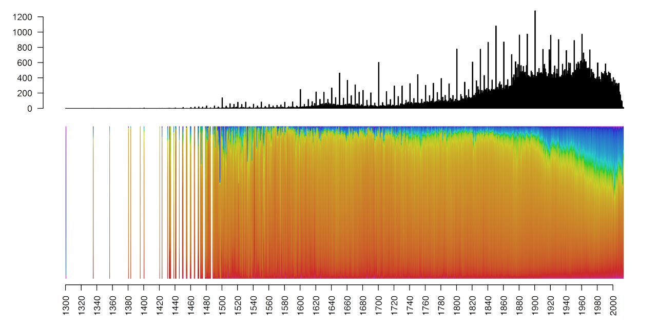
sum(npics)

This is based on a total of 120 013 images. I added a histogram on the top to show the number of images used for each year. The spikes at each decade might be because the uncertain dating was registered as an even decade.

The majority of paintings are painted between 1800 and 2000. Therefore, let us zoom in on that period.

par("mar"= c(4, 0, 0, 0) + 0.1)
plot(1:(length(1800:2000)+1),type="n", bty="n", xaxt="n", yaxt="n",xlab="", ylab="")
axis(1, at=(1:length(1800:2000))[1800:2000 %in% seq(1800,2000,10)], labels=seq(1800,2000,10),las=2, lwd=0, lwd.tick = 1, cex.axis=1.2)
 
for (k in 1:length(match(1800:2000,min(sort.years):max(sort.years)))) {
 
 if(length(newH[[match(1800:2000,min(sort.years):max(sort.years))[k]]])!=0){
 tempc=sort(newH[[match(1800:2000,min(sort.years):max(sort.years))[k]]])
 tempc=c(tempc[tempc>280],tempc[tempc<=280])
   
 gradient.rect(k-0.5,1,k+0.5,length(1800:2000)+1,col=hex(HSV(tempc,0.8,0.8)),gradient="y",border=NA)
 }
}
 
sum(sapply(newH[match(1800:2000,min(sort.years):max(sort.years))],length)/px.sample)

Here is the same plot for the period 1800-2000. This is based on 94 526 images.

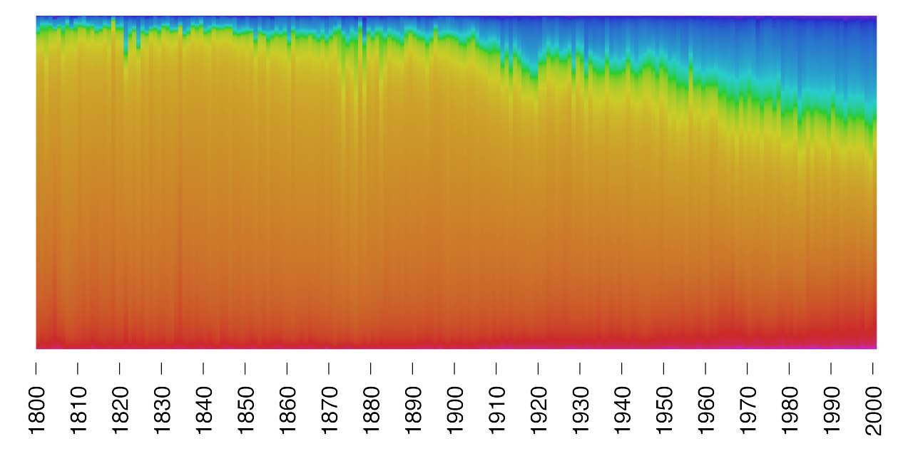
There seems to be a reliable trend of increasingly blue paintings throughout the 20^th century! Actually almost all colors seem to increase at the expense of orange. But let’s focus on the increase of blue.

The most popular proposed explanation for this trend among my friends and on social media seems to be:

The color blue is a relatively new color word (see: http://uk.businessinsider.com/what-is-blue-and-how-do-we-see-color-2015-2)
An increase in dark colors / black might drive the effect if these contain more blue or if the camera register them as blue to a larger extent.
The colors in paintings tend to change over time, e.g. due to the aging of resins (see: http://andbeyond.ch/Dissertation/Publications/J_Cult_Herit_2009_10_30-40.pdf)
Blue has historically been a very expensive color, and the decreasing price and increased supply might explain the increased use

Although interesting, I find the first explanation the least likely. Blue might be new, but not as new as the 1800s. Look for example at the presence of the word blue in 19^th and 20^th century books in Google Ngram viewer. However it definitely seem to have increased in frequency relative to other common color words.

Since these plots of colors ignore the Saturation and Value (in the HSV representation of the colors), we can also visualize how these change over time to see if it is the case that darkness increase over time.

plot(1:(length(1800:2000)+1), type="n", bty="n", xaxt="n", xlab="", ylab="", family="Helvetica", ylim=c(0,1), cex.axis=1.2)
axis(1, at=(1:length(1800:2000))[1800:2000 %in% seq(1800,2000,10)], labels=seq(1800,2000,10), las=2, lwd.tick = 1, family="Helvetica", cex.axis=1.2)
 
lines(sapply(all.S, mean)[sort.years %in% 1800:2000], type="l", col="grey60", lty=1, lwd=2)
lines(sapply(all.V, mean)[sort.years %in% 1800:2000], type="l", lty=1, lwd=2)
 
legend("topright",c("Saturation","Value"), col=c("grey60", "black"), lty=c(1, 1), bty="n", pch=16)

Looks like the colors are getting brighter over time, which speaks against the effect being driven by an increased use of dark colors or black.

The third suggestion is probably a better candidate. Although, if this is true, why does the apparent linear decay of blue suddenly stop? But maybe different blue pigments fade to different degrees and rates, and older paintings used more lasting pigments?

By sorting out the different techniques used in these paintings, we can investigate if the amount of blue in acrylic paintings also change over time. Out of the 121 312 paintings fed into the analysis (1299 of these were excluded from analysis, but let us ignore that for now) 110042 used oil, 5442 acrylic, 1035 tempera, and 4793 other/mixed.

Let’s look at the plot with only the acrylic paintings, to see if we get a different pattern.

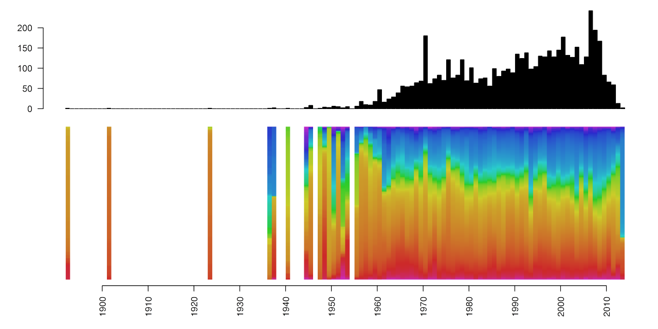
This result is based on 5250 acrylic paintings. Here there is no clear trend of increasing blue from the 1960s to the 2000s! Also the amount of blue is much larger in these images.

And the result from only the oil paintings is here:

Removing the other techniques does not change the pattern for the oil paintings. This plot is based on 109 209 images.

I haven’t found any data on the prices of blue, so that explanation is hard to elaborate on. However, it is not only blue that increases but all colors except orange, which might speak against the pigment prices explanation.

Of course the changes in color might be a results of a combination of factors. One of these could of course be trends in the use of color. If we assume a smooth linear deterioration of certain colors in oil paintings, it would be possible to subtract that change and study the short term fluctuation in color use. For example the marked increase of blue at the time of the First World War, might actually reflect a true trend in color use.

One obvious limitation here is that I have no information on the quality of the photographs of the paintings. The quality of the photos could potentially correlate with the years they were painted.

The BBC archive contain mostly British paintings and almost exclusively European paintings. It would be very interesting to find images from a broader range of countries to see how color use evolved in different cultures. Comparing trends between cultures might then also be a way of controlling for the mere effect of aging of the paint.

If you have any ideas of further analyses or questions, leave a comment!