Rockstars or Flop-stars? Examining Recruit Ratings and NFL Draft Success


College football recruiting is quickly becoming a billion-dollar business. Since the NCAA's ruling in the summer of 2021, there's been an explosion of valuations and incentives for young men and women across the country to trade their name, image and likeness (NIL) for brand advertising. Local businesses, from car dealerships to chicken joints, can offer payment to a student-athlete in exchange for their NIL in advertising campaigns. Schools and alumni associations can also band together to form "collectives," which can offer NIL contracts to student-athletes as long as the individual is not bound to the school and the school does not sanction the donation.
Simply put: NIL has created a veritable wild west of evaluating, recruiting and securing athletic talent. Many argue that this system is good on balance – student-athletes can finally expect fair compensation for their efforts and previously shady backroom deals are now dealt with in the open. Others see a slippery slope where College football becomes the NFL (or worse) and recruiting success only continues to consolidate among the most powerful programs. Regardless, as this new landscape allows 17-year-old boys to drive Lamborghinis to prom in $800 Dior high tops, it could also expose gaps in our ability to evaluate and target the right high-school talent.
After all, if you paid a cool $8 million to a junior in high school, you would probably like some certainty that they will produce for your school and go on to represent them in the NFL.
With this in mind, our objective is to examine how well composite recruit ratings supplied by 24/7 sports predict a player's likelihood of NFL draft success. We will define draft success subjectively as being drafted in the first three rounds.
As a statistician and epidemiologist by training (Go UAB Blazers!), I believe we can test this directly. With any good experiment, however, there are four key assumptions and limitations that need to be stated:
- The data presented are adequate reflections of reality - we are humans and errors of data entry can occur.
- "Success" is defined arbitrarily. One could argue being drafted at all represents success as it is accomplished by only about 1% of college football players.
- Player metrics included a simplified, boiled down measure of player value added – Predicted Points Added (PPA) totaled over career and yearly average. Any time production is simplified like this we lose some explanatory power in our models at the expense of a simpler, cleaner analysis.
- All models and inferences are exploratory in nature - I do not claim to be an authority in college football recruiting and player evaluation. These data represent the start of a conversation, not its end.
Data:
Our data were extracted from Bill's CFB data API and merged to derive a final analytical set. Please go to my Github repository for all code used to generate these datasets and support this analysis. Here's a snapshot of the final training data frame:
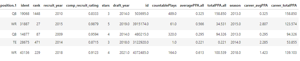
After significant data management, we derived a data frame with n=439 recruits that also contained records on CFB data for advanced player metrics. This dataset includes a player's name, position, college choice, composite recruiting rating, star rating, draft grade, draft round and a few predicted points added (PPA) metrics for collegiate performance markers.
Some feature engineering (one-hot encoding) was conducted on our data to allow for Logistic and Random Forest modeling.
Recruiting over time:
College football recruiting used to be like electoral primaries – decisions and deals were made in smoky back rooms not visible to the public. Speculation by reporters and message boards in recruiting season used to be relegated to a few short, intense months out of the year. We flipped open our Motorola Razors or booted up our AOL Instant Messager to see the latest on a prized running back out of Florida or gunslinger out West. But with Twitter, NIL, and the transfer portal, recruiting is now a year-round sprinted marathon.
How have recruit ratings changed in this time, if at all? And do these ratings matter to draft success as we've defined it?


Descriptive analysis of our recruits suggests some interesting trends:
- Overall, variance in recruit ratings for draftees in rounds 1-3 decreased over time
- Average rating of successful draftees remained relatively stable
- After 2010, successfully drafted recruits had consistently higher average composite ratings
- Advanced player metrics (career total PPA) appear to at least modify some of the relationship between recruit rating and draft success (pictured below)
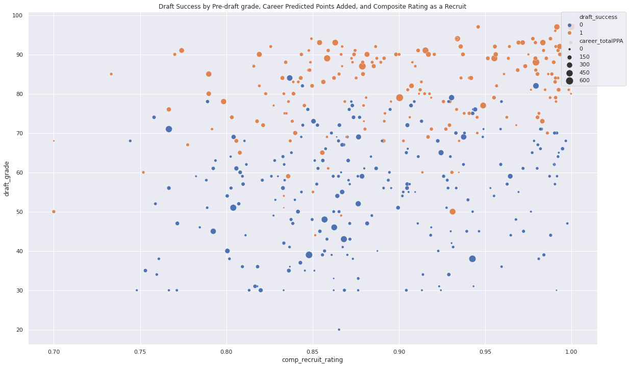
We also found that the only strong correlate of draft success was draft grade – no other metrics or ratings rose above moderate correlation (r > 0.4-0.5). This could make constructing an accurate model difficult, but that result could still provide some interesting points of discussion.
Predicting Draft Success:
Answering our initial question of draft success from recruiting data will require some statistical modeling. Fortunately, the nice folks at collegefootballdata.com have graciously created an open-source API to get your hands on GBs of data to answer all of your CFB nerd questions.
Logistic Model:
With the aim of parsimony (i.e., providing the clearest answer in the simplest way possible) we should first model draft success by logistic regression. A logistic regression assumes a binary outcome (0 or 1) and examines the likelihood of change in that outcome by each explanatory variable. So in our example, we want to look at how well recruit ratings, with some other potential explanatory variables held constant, predict being drafted in the first three rounds. This can be explained mathematically simply as:
Logit (Draft success = 1) = Recruit rating + Metrics + Demographics
And we can implement it in Python by the following:
from sklearn.linear_model import LogisticRegression
import warnings
warnings.filterwarnings('ignore')

logreg = LogisticRegression(random_state=9, max_iter = 200)

# fit the model with data
logreg.fit(OH_X_train, y_train)

y_pred = logreg.predict(OH_X_valid)

print('Logistic model converged and fit.')
Then build our confusion matrix and ROC curves– metrics which answer how well our model predicted actual data versus training data– and assess performance:
from sklearn import metrics
import numpy as np
import matplotlib.pyplot as plt
import seaborn as sns

cnf_matrix = metrics.confusion_matrix(y_valid, y_pred)
cnf_matrix

class_names=[0,1] # name  of classes
fig, ax = plt.subplots()
tick_marks = np.arange(len(class_names))
plt.xticks(tick_marks, class_names)
plt.yticks(tick_marks, class_names)

# create heatmap
sns.heatmap(pd.DataFrame(cnf_matrix), annot=True, cmap="YlGnBu" ,fmt='g')
ax.xaxis.set_label_position("top")
plt.tight_layout()
plt.title('Confusion matrix', y=1.1)
plt.ylabel('Actual label')
plt.xlabel('Predicted label')

plt.show()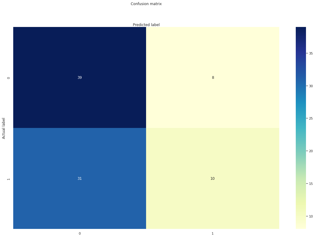
import warnings
warnings.filterwarnings('ignore')

y_pred_proba = logreg.predict_proba(OH_X_valid)[::,1]
fpr, tpr, _ = metrics.roc_curve(y_valid,  y_pred_proba)
auc = metrics.roc_auc_score(y_valid, y_pred_proba)
plt.plot(fpr,tpr,label="Logistic Model - all predictors, auc="+str(auc))
plt.legend(loc=4)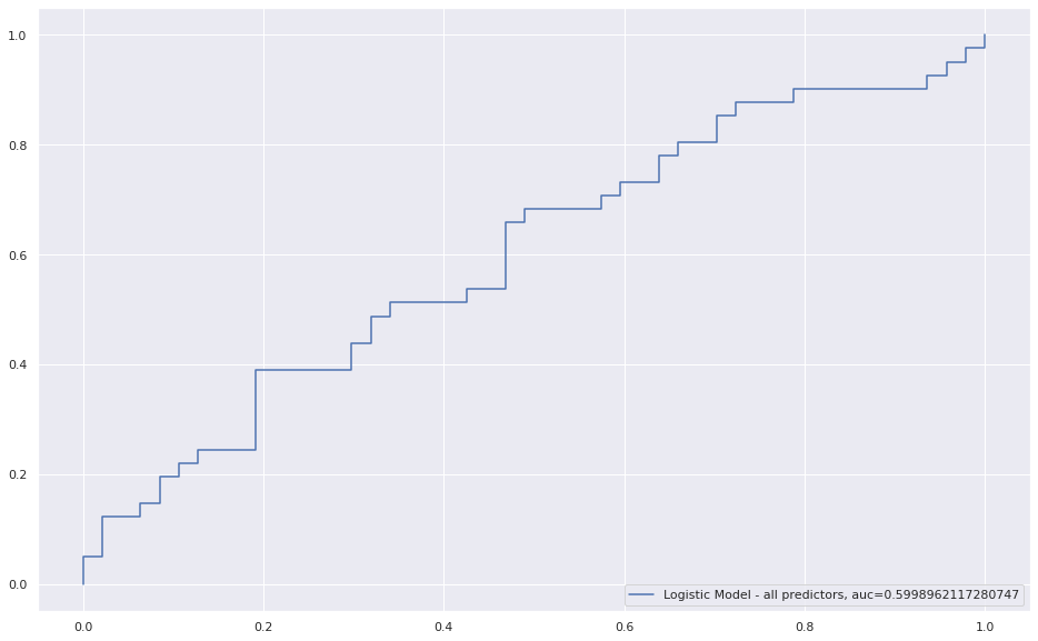
Random Forest:
Given a relatively poor performance of our logistic model (60%), we are warranted to try and beef up our predictive power with a Random Forest regression. The goal of an RF model is similar to a logistic model: to classify a binary outcome given some set of data. It is a machine learning algorithm which iteratively compare decision "trees" of data to arrive at the best classifier of the outcome. We will avoid the mathematical arguments for now, but safely assert its mechanics are more complex than the logistic model. This is one of the tradeoffs with RF models – it sacrifices some "explain-ability" for accuracy in prediction. With the necessary caveats out of the way, let's build our first RF model:
from sklearn.ensemble import RandomForestClassifier
from sklearn import metrics

#Create Classifier
clf=RandomForestClassifier(n_estimators=100)

#Train the model using the training sets
y_pred=clf.predict(X_test)
clf.fit(OH_X_train, y_train)

y_pred=clf.predict(OH_X_valid)

# Model Accuracy, how often is the classifier correct?
print("Accuracy:",metrics.accuracy_score(y_valid, y_pred))
Accuracy: 0.579 – marginally lower than our logistic model.
If we modified features further for a second model, we might want to trim based on feature importance. This can be accomplished by printing the automatically computed feature importance from the RF classifier in sklearn.
#set up the classifier:
RandomForestClassifier(bootstrap=True, class_weight=None, criterion='gini',
            max_depth=None, max_features='auto', max_leaf_nodes=None,
            min_impurity_decrease=0.0,
            min_samples_leaf=1, min_samples_split=2,
            min_weight_fraction_leaf=0.0, n_estimators=100, n_jobs=1,
            oob_score=False, random_state=None, verbose=0,
            warm_start=False)

#print feature importance:
feature_imp = pd.Series(clf.feature_importances_,index=OH_X_train.columns).sort_values(ascending=False)
feature_impResults: career_totalPPA = 0.114, totalPPA = 0.109, composite recruit rating = 0.090, averagePPA = 0.088
%matplotlib inline
# Creating a bar plot
sns.barplot(x=feature_imp, y=feature_imp.index)

sns.set(rc={"figure.figsize": (28, 14)})

# Add labels to your graph
plt.xlabel('Importance Score (Gini)')
plt.ylabel('Features')
plt.title("Feature Importance to Draft Success")
plt.legend()
plt.show()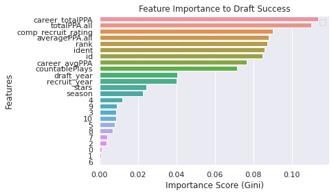
We might then drop what we don't find valuable to the model and rebuild our classifier.
X_trimmed = OH_X_train.drop(['ident', 'id', 'season', 'recruit_year'], axis = 1)
X_valid_trimmed = OH_X_valid.drop(['ident', 'id', 'season', 'recruit_year'], axis = 1)

clf=RandomForestClassifier(n_estimators=100)

clf.fit(X_trimmed,y_train)

y_pred=clf.predict(X_valid_trimmed)

print("Accuracy:",metrics.accuracy_score(y_valid, y_pred))
Accuracy: 0.591 - a moderate improvement over our first RF model.
Conclusions:
In our exploration of College Football Recruiting and NFL draft data from 2009-2018, we found that a player's composite recruiting rating was not an important predictor of draft success. Other findings are worth noting. Advanced player metrics across a career, their countable plays (i.e., player usage) and even the year of their recruitment were reasonable predictors of draft success. Modeling accuracy remained moderate at best, suggesting either the need for incorporating a more complete range of data or additional variables in subsequent analyses. Future analyses might also redefine draft success (as drafted in any round versus the first three) and incorporate different methods for feature engineering.
Predicting any human behavior is complex. Predicting how a 17-year-old boy will perform for the next 5-7 years is nearly impossible. But with round-the-clock agencies and scouts entering the Moneyball era, player evaluation could become even more nuanced and important to the landscape of recruiting and attracting talent. If anything should be taken from our analysis, it is that predicting a player's chance at the NFL would be better served by the breadth and depth of their collegiate experience and performance, rather than their prospects as a collegiate recruit inking million-dollar deals.