
College Basketball Rating (CBR): A new body-of-work metric for NCAA tournament selection
Abstract
The 2018-2019 NCAA men’s basketball tournament featured 32 automatic qualifiers and 36 at-large selections. A new metric, College Basketball Rating (CBR), agrees with 30 of the 36 at-large selections but disagrees with the other six teams. CBR finds St. John’s, Temple, Seton Hall, Ole Miss, Baylor, and Minnesota unworthy of an at-large selection and instead prefers Clemson, Texas, Lipscomb, Nebraska, NC State, and TCU. In the most extreme case, CBR identifies 45 non-tournament teams more deserving of an at-large selection than St. John’s. This paper highlights the numerous benefits of CBR and presents strong evidence in favor of its use in determining future NCAA tournament at-large selections.
1Introduction
The week leading up to the start of the NCAA men’s basketball tournament is action-packed. Conference championships are held, the selection committee releases the list of tournament teams, pundits analyze every selection, and fans rush to fill out their brackets before the play-in games start. Of the 68 teams who qualify for the tournament, 32 get in by winning their conference tournament and the remaining 36 are selected at-large by the committee. The ten-person committee relies on data from many different sources, both qualitative (“eye test”, injuries, etc.) and quantitative (box score stats, advanced metrics, etc.), when evaluating the resume of each team (NCAA, 2019). Among the most commonly discussed advanced metrics are ESPN’s basketball power index (BPI), Ken Pomeroy’s KenPom rankings, and the NCAA evaluation tool (NET).
Some metrics (like BPI and KenPom) and related analyses are designed to predict a team’s likelihood of winning future games (Glickman and Sonas, 2015; Steinberg and Latif, 2018). Others aim to predict which teams will be selected by the committee (Coleman, DuMond, and Lynch, 2016; Dutta and Jacobson, 2018; Reinig and Horowitz, 2019).
College Basketball Rating (CBR) belongs to neither category; it is a metric designed to compare bodies of work and determine which teams should be selected by the committee. It shares some things in common with today’s most popular advanced metrics, but in many ways CBR is unique. It requires only box score stats, and the finished product is a number that is simple, transparent, accurate, and fair.
As shown in Table 1, CBR shares some things in common with BPI, KenPom, and NET. CBR and KenPom both place little emphasis on wins and have a soft cap for point margin (Pomeroy, 2013). CBR and NET both assume nothing about a team before the start of the season (Katz, 2019). However, CBR is unique in that it does not use possession-level efficiency calculations and sometimes assumes the loser of a game played better than the winner.
Table 1
Comparison of CBR to BPI, KenPom, and NET
| Metric | Type | Accounts for Preseason Info | Emphasizes Win % | Point Margin Cap |
| BPI | Predictive | Yes | Yes | None |
| KenPom | Predictive | Yes | No | Soft |
| NET | Blended | No | Yes | Hard |
| CBR | Descriptive | No | No | Soft |
2Methodology
2.1Data
Game-level data comes from the Team Game Finder at sports-reference.com/cbb. It includes 5,909 college basketball games from the 2018-2019 regular season where at least one of the teams belongs to NCAA Division I. The data includes the conference tournaments and excludes the end-of-year NCAA and NIT tournaments.
2.2Game Score Definition
The foundation of CBR is built upon the concept of “game score”. Game score is a continuous number between 0 and 1 that represents a team’s performance in a game; 0 and 1 represent total domination on both the offensive and defensive ends of the court (0 if loser; 1 if winner), and 0.5 represents a close game in which teams were evenly matched. A fitted value is generated using logistic regression, a common statistical modeling technique in which explanatory variables are evaluated based on their ability to move the needle between a binary outcome (Cramer, 2002). The fitted value then goes through a correction to dampen the effect of outlier performances and becomes a game score.
2.3Logistic Model
The explanatory variables used in the logistic model are offensive rebounds (ORB), defensive rebounds (DRB), assists (AST), steals (STL), blocks (BLK), turnovers (TOV), personal fouls (PF), field goals attempted (FGA), and free throws attempted (FTA). All variables are represented as the difference relative to the opponent. For example, if a box score shows five steals for Team A and eight steals for Team B, the steals variable is – 3 for Team A and +3 for Team B. The binary response variable is 0 for the loser of the game and 1 for the winner.
The logistic model summary is shown in Table 2. The coefficients for defensive rebounds, assists, steals, blocks, field goals attempted, and free throws attempted indicate a positive relationship with winning the game. The coefficients for offensive rebounds, turnovers, and personal fouls indicate a negative relationship with winning the game. For rebounds, the logistic model believes a defensive rebounding advantage is good because the opponent is missing shots and an offensive rebounding advantage is bad because the team in question is missing shots.
Table 2
Logistic Model (Response Variable is 0 for Loser and 1 for Winner)
| Explanatory Variable | Coefficient | Standard Error | Test Statistic | P-Value |
| Offensive Rebounds | – 0.075 | 0.017 | – 4.47 | <0.0001 |
| Defensive Rebounds | 0.379 | 0.013 | 29.67 | <0.0001 |
| Assists | 0.147 | 0.009 | 16.42 | <0.0001 |
| Steals | 0.014 | 0.014 | 1.00 | 0.3196 |
| Blocks | 0.056 | 0.013 | 4.32 | <0.0001 |
| Turnovers | – 0.345 | 0.019 | – 18.47 | <0.0001 |
| Personal Fouls | – 0.098 | 0.014 | – 7.07 | <0.0001 |
| Field Goals Attempted | 0.031 | 0.014 | 2.11 | 0.0347 |
| Free Throws Attempted | 0.072 | 0.010 | 7.13 | <0.0001 |
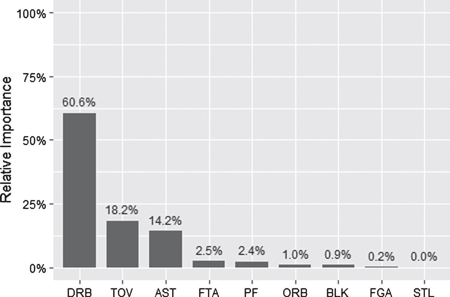
Which box score stat is the most consistent predictor of the outcome? Shown in Fig. 1 is the relative importance of the explanatory variables in the logistic model. For a given variable, importance is defined as the difference in residual deviance (a measure of unexplained variation) for the full model versus a nested model in which that variable is excluded. For example, when all variables are included, the residual deviance is 4,728. When all variables except defensive rebounds are included, the residual deviance jumps to 5,998. When all variables except steals are included, the residual deviance barely increases to 4,729. Since the exclusion of defensive rebounds has the most dramatic effect on the residual deviance, it is deemed the most “important” variable.
Fig. 1
Logistic Model – Relative Importance of the Explanatory Variables.
Fitted values for the logistic model are calculated using the formula shown above. The betas β1, β2, …, β9 are the coefficients from Table 2.
The logistic model classifies 91% of win/loss outcomes correctly. The remaining variation unexplained by the model can be mostly attributed to shooting percentage. For example, if a team takes 25 threes in a game, whether they make 45% versus 20% of those shots has a huge impact on the outcome. Shooting percentage is intentionally left out of the model, with the assumption that non-shooting stats are more representative of team strength since shooting percentage is noisy (players and teams go through hot and cold streaks).
2.4Justification for the Logistic Model
To determine whether the logistic model is an appropriate choice for this dataset, two competitor models are considered. The first competitor model is a support vector machine (SVM). SVM is a common classification technique in which a hyperplane is drawn in n-dimensional space to separate the response variable. It performs well on small, non-noisy datasets such as this one.
The second competitor model is a gradient-boosted machine (GBM). GBM is an advanced machine learning technique in which many weak models (decision trees) are combined to create a strong one. It can produce highly accurate predictions as long as there is minimal overfitting on the training set. To strike this balance between bias and variance, GBM uses two primary techniques: boosting and bagging. Boosting puts added emphasis on hard-to-predict areas while bagging subsamples the data to produce robust parameter estimates.
70% of the dataset is used to train the model and the remaining 30% is used to test its performance. Five-fold cross validation is performed to help minimize overfitting and a grid search algorithm is used to determine the hyperparameters that minimize the prediction error on the test set. The optimal SVM model has a polynomial kernel and a cost of four, while the optimal GBM model has 225 trees, an interaction depth of two, and a learning rate of 0.1.
Shown in Table 3 is a comparison of the logistic model versus its two competitors. The accuracy metric, area under the ROC curve, measures a model’s performance across different classification thresholds and estimates the probability that a randomly chosen winning team has a higher predicted value than a randomly chosen losing team (Google, 2020). Note that the logistic model performs best on the test set as well as on regular season data from the following year.
Table 3
Area Under the ROC Curve – Logistic Model vs. SVM/GBM
| Model | 70% Training Set | 30% Test Set | 2019-2020 Season |
| Logistic | 0.969 | 0.969 | 0.971 |
| SVM | 0.968 | 0.966 | 0.962 |
| GBM | 0.970 | 0.966 | 0.968 |
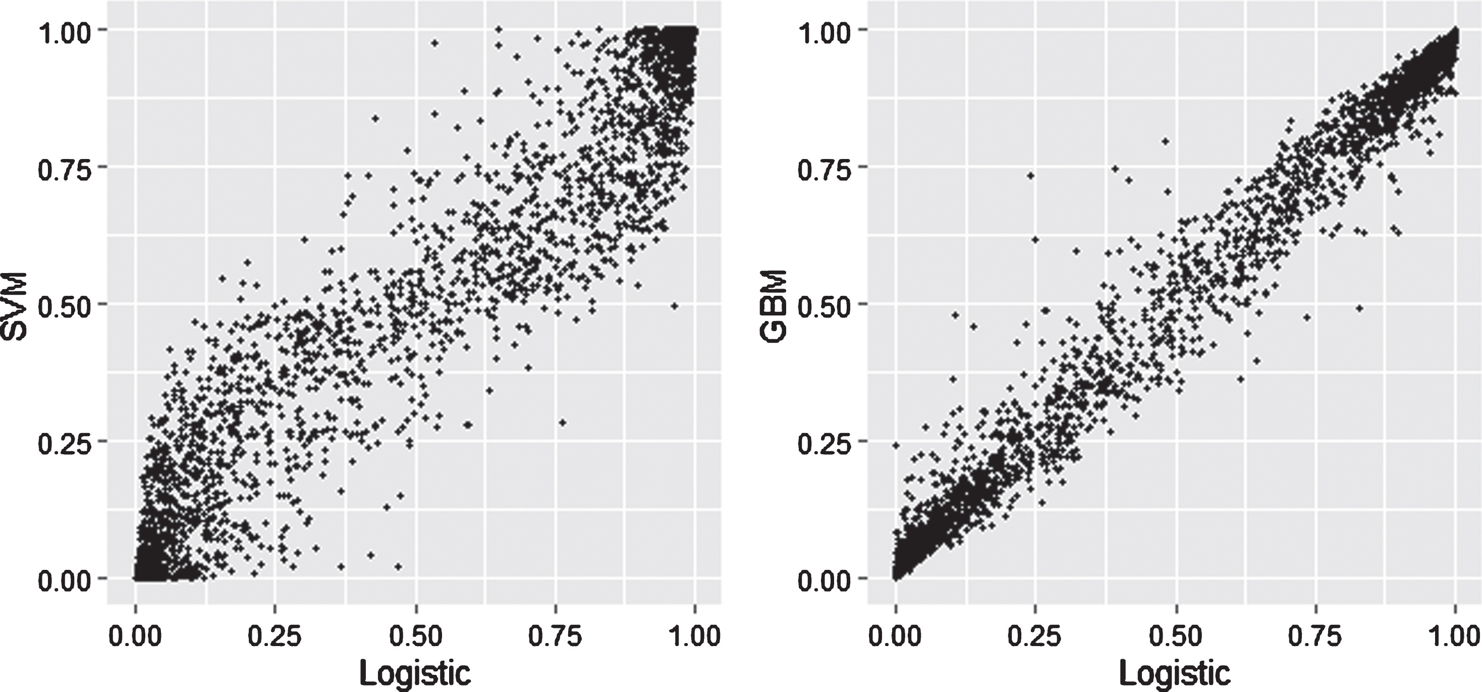
Shown in Fig. 2 is a comparison of predicted values on the test set for the logistic model versus SVM and GBM. Note that there is strong agreement between the models when 0.5 is used as the classification threshold.
Fig. 2
Test Set Predictions – Logistic vs. SVM and GBM.
Regarding predictive accuracy, 88% of outcomes in the test set are classified correctly by all three models and 8% are classified incorrectly by all three models. The remaining 4% are cases in which one of the models disagrees with the other two. The game with the highest variance between the three predictions is Georgia Tech’s 73-65 home win over Pitt on 2/20/2019. Despite attempting nine more field goals and 14 more free throws, Pitt found a way to lose by allowing 11 more blocks and going 20-38 from the free throw line.
Ultimately, the logistic model is chosen for its predictive accuracy (does not overfit the data) and its interpretability. It is not only the most accurate of the three models by a slight margin, but also the simplest and most transparent.
2.5Game Score Calculation
The logistic model generates a fitted value for each team per game. Given the known positive relationship between home-court advantage and box score stats (Bommel, Bornn, Chow-White, and Gao, 2019), the fitted value is then corrected following the rules shown in Table 4.
Table 4
Game Score Bounds by Adjusted Point Margin (+3 if Away; – 3 if Home)
| Adjusted Point Margin | Game Score Lower Bound | Game Score Upper Bound |
| – 30+ | 0 | 0 |
| – 25 to – 29 | 0 | 0.1 |
| – 20 to – 24 | 0 | 0.2 |
| – 15 to – 19 | 0.1 | 0.3 |
| – 10 to – 14 | 0.2 | 0.4 |
| – 5 to – 9 | 0.3 | 0.5 |
| – 4 to 4 | 0.4 | 0.6 |
| 5 to 9 | 0.5 | 0.7 |
| 10 to 14 | 0.6 | 0.8 |
| 15 to 19 | 0.7 | 0.9 |
| 20 to 24 | 0.8 | 1 |
| 25 to 29 | 0.9 | 1 |
| 30+ | 1 | 1 |
For example, if a team’s location-adjusted point margin (+3 adjustment if away team; – 3 adjustment if home team) is between – 4 and 4, the game score must be between 0.4 and 0.6. The reasoning is that even if a team plays poorly (for example, many turnovers and few assists), if the final score is close that team should not be punished too severely. The correction strikes a nice balance between the non-shooting effects from the logistic model and the reasonable qualitative inference that is made about the relative skill level of two teams based on the score of the game.
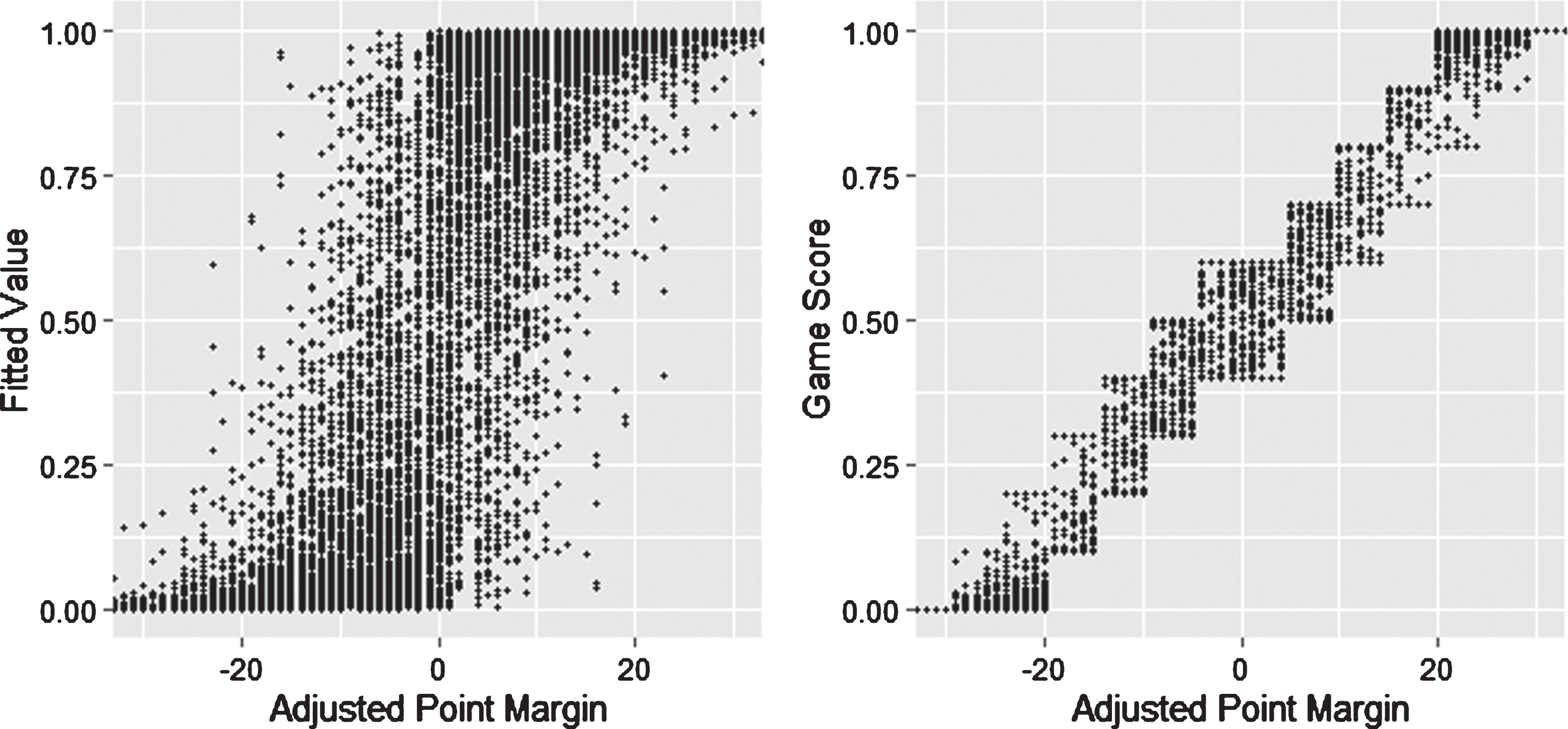
As shown in Fig. 3, the correction dampens the effect of outlier non-shooting performances while still allowing for some variability between game outcomes that look similar on paper. For example, if a home team wins by nine points or an away team wins by three points, both teams have an adjusted point margin of +6. Based on the correction, an adjusted point margin of +6 corresponds to a game score between 0.5 and 0.7. Whether the game score is set to 0.5, 0.7, or something in between depends on that team’s non-shooting performance in the game.
Fig. 3
How the Adjusted Point Margin Correction Turns a Fitted Value Into a Game Score.
2.6Game Score Example: Duke vs. Syracuse
For a better understanding of how game score is calculated, consider Duke’s 91-95 overtime home loss to Syracuse on 1/14/2019. Duke lost by four points at home, so the adjusted point margin is – 7 for Duke and +7 for Syracuse. Due to the correction, Duke’s game score must be between 0.3 and 0.5 and Syracuse’s game score must be between 0.5 and 0.7.
As shown in Table 5, Duke dominated the non-shooting categories with eight more assists, five more steals, seven more blocks, three fewer turnovers, and eight more free throw attempts than Syracuse. The deciding factor in the game was Duke going 9-43 (21%) from beyond the arc versus Syracuse’s 11-25 (44%). Although they lost, the logistic model considers Duke’s three-point shooting an outlier performance and gives credit to Duke as if they dominated the game.
Table 5
Duke (91) vs. Syracuse (95) – Game Score Calculation
| Statistic | Duke | Syracuse |
| Offensive Rebounds | 3 | – 3 |
| Defensive Rebounds | 1 | – 1 |
| Assists | 8 | – 8 |
| Steals | 5 | – 5 |
| Blocks | 7 | – 7 |
| Turnovers | – 3 | 3 |
| Personal Fouls | 0 | 0 |
| Field Goals Attempted | 0 | 0 |
| Free Throws Attempted | 8 | – 8 |
| Fitted Value | 0.97 | 0.03 |
| Point Margin | – 4 | 4 |
| Adjusted Point Margin | – 7 | 7 |
| Game Score | 0.50 | 0.50 |
The logistic model gives Duke a fitted value of 0.97 and Syracuse a fitted value of 0.03. After the correction, Duke’s game score is 0.5 and Syracuse’s game score is also 0.5. The post-correction interpretation is that Duke dominated the game in the non-shooting categories but Syracuse won by four points on the road. The logistic model combined with the adjusted point margin correction ultimately gives these teams equal credit for their performance in the game.
2.7Optimization of the System
With game scores calculated, the next step is to define the relationship between game score and CBR difference. The theory behind the CBR system is that every team has an unknown true coefficient representing their body of work relative to the other teams. The estimated coefficient, CBR, is the value that minimizes the error of the system when all teams and games are considered. A CBR of 0.00 represents a team with an average body of work.
Table 6 shows the linear relationship between game score and CBR difference. A game score of 0 corresponds to a CBR difference of – 5.00, a game score of 0.5 corresponds to a CBR difference of 0.00, and a game score of 1 corresponds to a CBR difference of 5.00. Because game score is always between 0 and 1, the system attempts to keep teams who have played each other within a CBR difference of – 5.00 to 5.00. As a result, CBR in rare cases punishes good teams for scheduling games against “cupcake” opponents. The most obvious example of a game in which CBR punishes the winner is Auburn’s 103-52 home win over Mississippi College on 11/14/2018.
Table 6
Game Score vs. CBR Difference
| Game Score | CBR Difference |
| 0 | – 5.00 |
| 0.1 | – 4.00 |
| 0.2 | – 3.00 |
| 0.3 | – 2.00 |
| 0.4 | – 1.00 |
| 0.5 | 0.00 |
| 0.6 | 1.00 |
| 0.7 | 2.00 |
| 0.8 | 3.00 |
| 0.9 | 4.00 |
| 1 | 5.00 |
Optimization of the system occurs in an iterative, deterministic way similar to maximum likelihood estimation (MLE). During a given iteration, if the average CBR difference between a team and its opponents is too high or low relative to its game scores, the estimate moves up or down to the break-even point. This does not immediately minimize the error of the system because the CBRs of other teams are being adjusted at the same time. After multiple iterations, however, the system finds equilibrium.
3Results
When the system reaches equilibrium, the distribution of ratings is roughly between – 10.00 and 5.00. CBR represents cumulative body of work, and related metrics easily calculated from CBR offer additional insight into a team’s season.
Table 7 shows the CBR top 10. There is strong agreement between CBR and the selection committee on who the top teams are.
Table 7
CBR Top 10
| Team | Record | CBR | CBR Rank | NCAA Tourn. Overall Seed |
| Duke | 29– 5 | 4.49 | 1 | 1 |
| Gonzaga | 30– 3 | 4.49 | 2 | 4 |
| Michigan State | 28– 6 | 4.48 | 3 | 6 |
| Virginia | 29– 3 | 4.44 | 4 | 2 |
| UNC | 27– 6 | 4.18 | 5 | 3 |
| Michigan | 28– 6 | 4.16 | 6 | 8 |
| Kentucky | 27– 6 | 3.92 | 7 | 7 |
| Tennessee | 29– 5 | 3.69 | 8 | 5 |
| Texas Tech | 26– 6 | 3.67 | 9 | 10 |
| Florida State | 27– 7 | 3.19 | 10 | 14 |
3.1Analysis of the Six At-Large Selection Discrepancies
CBR agrees with the selection committee on 30 of the 36 at-large selections. Of the six discrepancies, the CBR teams (Clemson, Texas, Lipscomb, Nebraska, NC State, and TCU) went 16-5 in the NIT tournament and the selection committee teams (St. John’s, Temple, Seton Hall, Ole Miss, Baylor, and Minnesota) went 2-6 in the NCAA tournament.
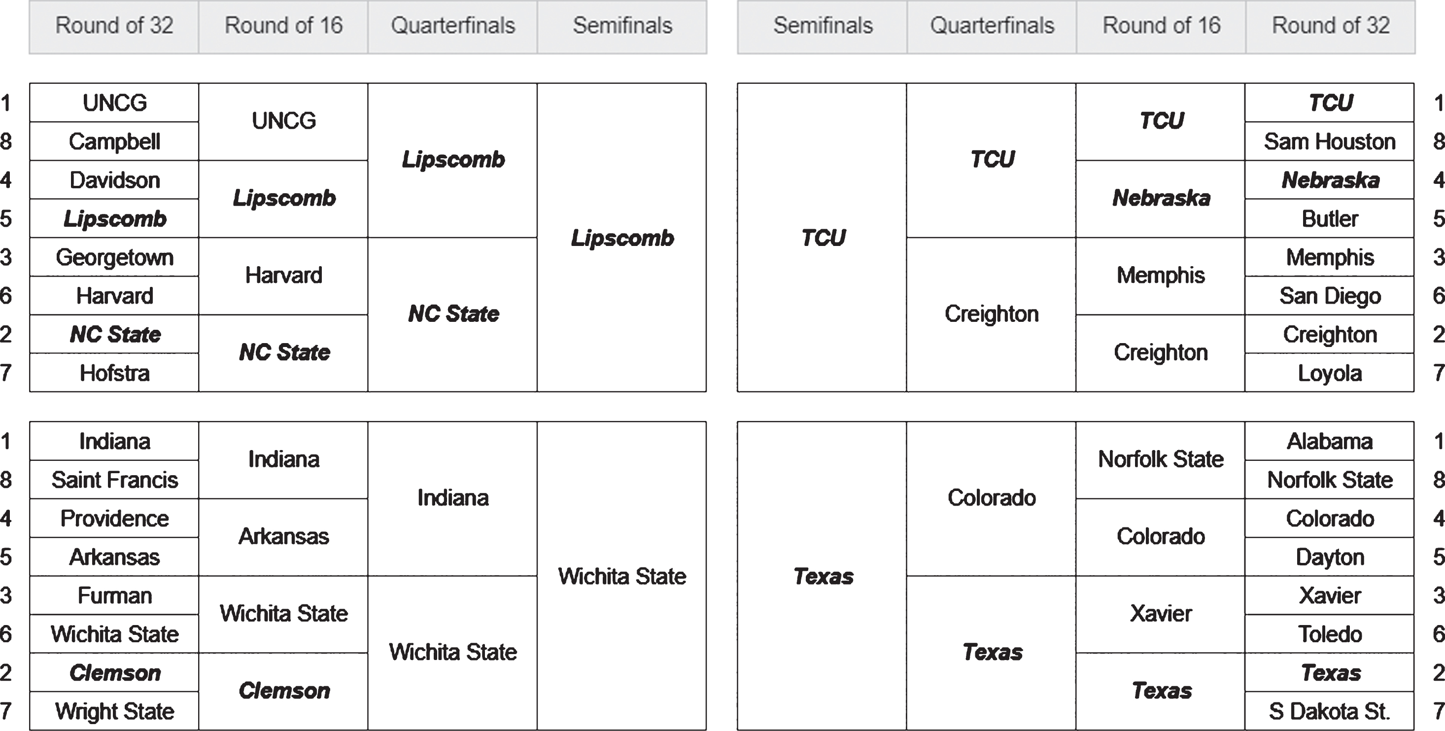
As shown in Fig. 4, the NIT semifinals featured Texas, Lipscomb, TCU, and Wichita State. Texas, a #2 seed, defeated Lipscomb, a #5 seed, in the final. These outcomes are noteworthy because they provide strong evidence in favor of CBR. Lipscomb, a team so far off the radar that it received a #5 seed in the NIT tournament, is an at-large NCAA tournament selection by a comfortable margin according to CBR.
Fig. 4
2018-2019 NIT Tournament (CBR Teams in Bold).
3.2Clemson vs. St John’s
The most noticeable discrepancy between CBR and the selection committee is St. John’s, a team CBR believes was less worthy than 45 non-tournament teams. Using CBR, a strong case can be made in favor of Clemson over St. John’s.
Table 8 shows Clemson’s 13 losses, six of which were within two points. The only double-digit losses Clemson had all year were against Duke (CBR #1), Virginia (CBR #4), Florida State (CBR #10), and Mississippi State (CBR #19). CBR gives credit to Clemson for these close losses and believes it should have been an at-large selection by a comfortable margin.
Table 8
Breakdown of Clemson’s 13 Losses
| Date | Location | Opponent | Point Margin | Game Score |
| 11/21/2018 | Neutral | Creighton | – 5 | 0.30 |
| 11/26/2018 | Home | Nebraska | – 2 | 0.46 |
| 12/8/2018 | Neutral | Miss. St. | – 11 | 0.20 |
| 1/5/2019 | Away | Duke | – 19 | 0.10 |
| 1/9/2019 | Away | Syracuse | – 8 | 0.30 |
| 1/12/2019 | Home | Virginia | – 20 | 0.02 |
| 1/22/2019 | Away | Florida State | – 9 | 0.30 |
| 1/26/2019 | Away | NC State | – 2 | 0.60 |
| 2/13/2019 | Away | Miami (FL) | – 1 | 0.60 |
| 2/16/2019 | Away | Louisville | – 1 | 0.40 |
| 2/19/2019 | Home | Florida State | – 13 | 0.10 |
| 3/2/2019 | Home | UNC | – 2 | 0.50 |
| 3/13/2019 | Neutral | NC State | – 1 | 0.40 |
Table 9 shows St. John’s 12 losses, ten of which were by eight points or more. St. John’s regular season ended with a 32-point loss to Marquette (CBR #28), while Clemson’s regular season ended with a one-point loss to NC State (CBR #41). St. John’s average game score in defeat is 0.21. Clemson’s average game score in defeat, against much better competition, is 0.33.
Table 9
Breakdown of St. John’s 12 Losses
| Date | Location | Opponent | Point Margin | Game Score |
| 12/29/2018 | Away | Seton Hall | – 2 | 0.40 |
| 1/8/2019 | Away | Villanova | – 5 | 0.40 |
| 1/12/2019 | Home | DePaul | – 8 | 0.20 |
| 1/19/2019 | Away | Butler | – 9 | 0.30 |
| 1/27/2019 | Home | Georgetown | – 11 | 0.27 |
| 2/2/2019 | Away | Duke | – 30 | 0.00 |
| 2/9/2019 | Home | Providence | – 14 | 0.10 |
| 2/20/2019 | Away | Providence | – 19 | 0.10 |
| 2/28/2019 | Home | Xavier | – 11 | 0.20 |
| 3/3/2019 | Away | DePaul | – 9 | 0.30 |
| 3/9/2019 | Away | Xavier | – 13 | 0.20 |
| 3/14/2019 | Neutral | Marquette | – 32 | 0.00 |
St. John’s resume also includes unconvincing wins over Maryland East Shore (CBR #407), Mount St. Mary’s (CBR #354), and Cal (CBR #266). Of St. John’s 13 wins against CBR 0.00 + teams, only four were by double digits. Of Clemson’s 14 wins against CBR 0.00 + teams, ten were by double digits.
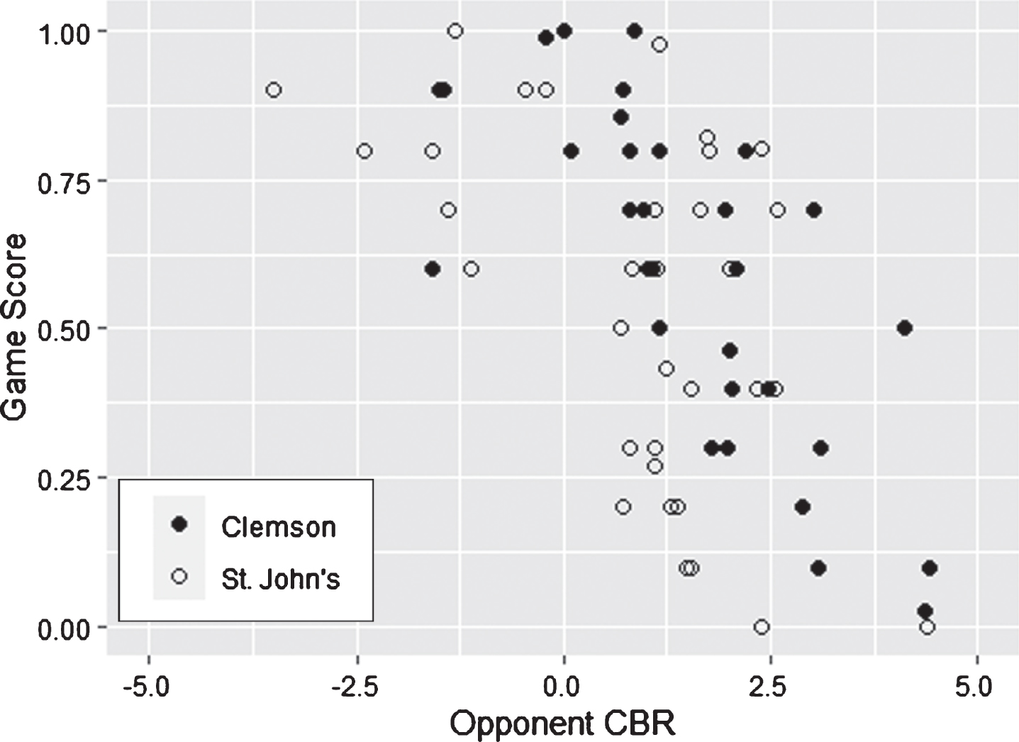
Figure 5 provides additional insight into CBR’s preference of Clemson over St. John’s. It shows a breakdown of game score by opponent CBR. For example, St. John’s played an opponent with CBR 4.39 and had a game score of 0. When their schedules are combined, Clemson played seven of the eight strongest opponents and St. John’s played eight of the 11 weakest opponents. The matches against opponents with a CBR of 0.00 to 2.50, however, offer the most convincing evidence in favor of Clemson. Against opponents in this tier, Clemson has an average game score of 0.65 and zero game scores under 0.30. St. John’s, on the other hand, has an average game score of 0.45 and seven game scores under 0.30. In this head-to-head comparison, CBR presents compelling evidence that Clemson played at a higher level against tougher competition.
Fig. 5
Game Score vs. Opponent CBR – Clemson vs. St. John’s.
3.3CBR vs. NET
The 2018-2019 college basketball season featured the debut of NET. Its first rankings, released on 11/26/2018, were met with heavy criticism for Ohio State at #1 (too high), Gonzaga at #5 (too low), Duke at #6 (too low), Loyola Marymount at #10 (too high), and Belmont at #12 (too high) (Baer, 2018). Much of the conversation centered around NET’s hard 10-point margin cap, its lack of punishment for beating cupcake teams, and its efficiency calculations that ignore strength of opponent.
CBR and NET both assume nothing about a team’s players, coaches, or pedigree; every season starts with a blank slate. By definition, these metrics are more valuable at the end of the season than the beginning. Early season CBR and NET rankings, however, do provide interesting insight into what types of teams and performances are favored by the algorithm.
Table 10 shows a comparison of CBR and NET using data through 11/25/2018. Note that CBR drops Ohio State from #1 to #5, bumps Gonzaga from #5 to #2, bumps Duke from #6 to #4, drops Loyola Marymount from #10 to #24, and drops Belmont from #12 to #60.
Table 10
Analysis of NET Top 12 – Data Through 11/25/2018
| Team | Record | NET Rank | CBR Rank |
| Ohio State | 6– 0 | 1 | 5 |
| Virginia | 6– 0 | 2 | 19 |
| Texas Tech | 6– 0 | 3 | 1 |
| Michigan | 6– 0 | 4 | 3 |
| Gonzaga | 6– 0 | 5 | 2 |
| Duke | 5– 1 | 6 | 4 |
| Michigan State | 5– 1 | 7 | 17 |
| Wisconsin | 5– 1 | 8 | 13 |
| Virginia Tech | 5– 0 | 9 | 6 |
| Loyola Marymount | 7– 0 | 10 | 24 |
| Kansas | 5– 0 | 11 | 12 |
| Belmont | 5– 0 | 12 | 60 |
4Discussion
When it comes to descriptive body-of-work metrics, too much emphasis is placed on wins and losses. The margin in college basketball is thin; games are often decided by a referee’s missed call or a few tenths of a second on the clock. As analytics continues to become a more central part of the mainstream discussion, perhaps the narrative will shift from “quadrant 1 wins” to “game score against above-average opponents”.
CBR is a modern body-of-work metric. It places minimal emphasis on high-variance outcomes like win/loss and shots made/missed, and instead focuses on box score stats that good teams accumulate consistently. CBR is unique because no other descriptive metric is as simple, transparent, and accurate.
CBR is calculated in three basic steps. First, a fitted value is generated from a logistic model that looks at non-shooting box score stats. Second, the fitted value receives a location-adjusted point margin correction and becomes a game score. Third, game scores are mapped to an expected CBR difference between opponents and iterative updates are performed until the error of the system is minimized. The finished product is a single number for each team that represents cumulative body of work relative to an average team in the system.
For all its benefits, CBR does have limitations. It does not differentiate between conference versus non-conference matchups or games played early in the season versus late. Future research may indicate a need to adjust for these factors. Tweaks to the logistic model, the adjusted point margin correction, and/or the minimization loss function may prove to add value to the system. CBR also does not account for win/loss. Adjustments may be necessary if close wins are determined to be correlated with future performance in pressure situations. Finally, it remains to be seen whether CBR is good at predicting the outcome of future games. It currently focuses only on quantifying cumulative body of work.
5Conclusion
Empirical evidence supports the claim that CBR should be considered when discussing a team’s body of work. For the 2018-2019 college basketball season, CBR identifies six discrepancies in the NCAA at-large selection process. Of the six discrepancies, the CBR teams played extremely well in the NIT tournament and the selection committee teams played poorly in the NCAA tournament.
For Clemson versus St. John’s, the selection committee may have preferred St. John’s due to its better overall, non-conference, and quadrant 1 records. These win/loss breakdowns are misleading and represent an old-school way of thinking about sports outcomes. CBR, a single number that represents a team’s game score distribution by opponent strength, tells a more accurate and complete story.
Acknowledgments
The author would like to thank the people at sports-reference.com for making sports data free and accessible for everyone.
References
1 | Baer, J. , (2018) , ‘Just about everyone is having issues with the NCAA’s new RPI replacement.’ yahoo.com. https://sports.yahoo.com/just-everyone-issues-ncaas-new-rpi-replacement-023810498.html [Accessed 23 December 2019]. |
2 | Bommel, M. , Bornn, L. , Chow-White, P. and Gao, C. , (2019) , ‘Home Sweet Home: Quantifying Home Court Advantages For NCAA Basketball Statistics.’ arXiv e-prints, arXiv:1909.04817. |
3 | Coleman, B. , DuMond, J. and Lynch, A. , (2016) , ‘An easily implemented and accurate model for predicting NCAA tournament at-large bids.’, Journal of Sports Analytics 2: (2), 121–132. |
4 | Cramer, J. , (2002) , ‘The Origins of Logistic Regression.’ Tinbergen Institute. https://papers.tinbergen.nl/02119.pdf |
5 | Dutta, S. and Jacobson, S. , (2018) , ‘Modeling the NCAA basketball tournament selection process using a decision tree.’ Journal of Sports Analytics 4: (1), 65–71. |
6 | Glickman, M. and Sonas, J. , (2015) , ‘Introduction to the NCAA men’s basketball prediction methods issue.’ Journal of Quantitative Analysis in Sports 11: (1), 1–3. |
7 | Google, 2020, ‘Classification: ROC Curve and AUC.’ developers.google.com. https://developers.google.com/machine-learning/crash-course/classification/roc-and-auc [Accessed 3 May 2020]. |
8 | Katz, A. , (2019) ,‘NET rankings: What to know about college basketball’s new tool to help select the NCAA tournament field.’ ncaa.com. https://www.ncaa.com/news/basketball-men/2018-08-22/net-rankings-what-know-about-college-basketballs-new-tool-help [Accessed 23 December 2019]. |
9 | NCAA, 2019, ‘How the field of 68 teams is picked for March Madness.’ ncaa.com. https://www.ncaa.com/news/basketball-men/article/2018-10-19/how-field-68-teams-picked-march-madness [Accessed 23 December 2019]. |
10 | Pomeroy, K. , (2013) , ‘Pomeroy Ratings version 2.0.’ kenpom.com. https://kenpom.com/blog/pomeroy-ratings-version-2.0/ [Accessed 23 December 2019]. |
11 | Reinig, B. and Horowitz, I. , (2019) , ‘Analyzing the impact of the NCAA Selection committee’s new quadrant system,’ Journal of Sports Analytics 5: (4), 325–333. |
12 | Steinberg, R. and Latif, Z. , (2018) , ‘March Madness Model Meta-Analysis: What determines success in a March Madness model?’ Pomona College. http://economics-files.pomona.edu/GarySmith/Econ190/Econ190%202018/MarchMadness.pdf |

