Modeling a Controlled-Floating Space Robot for In-Space Services: A Beginner’s Tutorial

1 Introduction

Innovative space system technologies have revolutionized the lives on Earth, which explains why the global space race continues. The space economy worldwide is booming, and there is now a paradigm shift to the in-orbit services and manufacturing (IOSM) market. There is a significant commercial boost in the in-orbit services market, which is predicted to be $1 billion by 2030 (Satellite Catapult Applications, Fair-Space and Astroscale, 2021). The candidate in-orbit missions include the following: servicing and repairing high-value space assets including operational spacecraft, life extension, refueling, orbit correction, in-space assembly of space telescopes for Earth observation and astronomical observations, space-based power generation, and active debris removal, to name a few (Oda et al., 1996; Whittaker et al., 2000; Yoshida, 2001; Friend, 2008; Shengwei, 2013; Flores-Abad et al., 2014; Jaekel et al., 2015; Lee et al., 2016; Reed et al., 2016; Medina et al., 2017; Taylor et al., 2018; Li et al., 2019; Wilde et al., 2019; Jackson et al., 2020; Nair et al., 2020; Romano, 2021; Xu, 2021). Building satellite servicing and debris removal capabilities will open up bigger and longer-term markets linked to assembly and manufacturing in space (Satellite Catapult Applications, Fair-Space and Astroscale, 2021). As the in-orbit economy evolves, robotics and autonomous systems will play a pivotal role in many future IOSM missions. However, controlling a space robot in an extreme environment is significantly more complex than its terrestrial counterpart; this is the foremost hurdle to the success of IOSM missions.

In the context of servicing a cooperative and noncooperative target spacecraft using a servicer space robot, safety is paramount during the close-range approach, target capture, and postcapture operations. Approaching a target spacecraft using a servicer space robot can be achieved by two different modes of operation: free-flying and free-floating (Dubowsky and Papadopoulos, 1993; Moosavian and Papadopoulos, 2007). The free-flying approach uses reaction jets to facilitate a stabilized and controlled base for the robot manipulator in motion. The stable platform is favorable for the manipulator’s motion, however, on the expense of excessive fuel consumption and limited workspace. On the other hand, the free-floating approach utilizes an uncontrolled base to limit fuel consumption on the expense of dynamic singularities and an undefined workspace for the robot. There is a well-established literature on these two modes of operation, and they have benefits depending on the nature of the mission (Longman et al., 1987; Papadopoulos and Dubowsky, 1991, 1993; Xu and Kanade, 1992; Xu, 1993; Yoshida and Abiko, 2002; Menon et al., 2007; Artigas et al., 2015; Guang et al., 2018; Wilde et al., 2018). For instance, when communication between the space robot and the ground station is paramount, the free-flying mode is preferred as its controlled base can keep the antennas pointing toward the Earth. On the other hand, when reducing fuel consumption is prioritized, the free-floating mode is more suitable because of its uncontrolled base. In addition, recent pertinent works include numerical simulations, hardware-in-the-loop experiments, and guidance algorithms to capture and detumble a space object (Virgili-Llop et al., 2017). Despite these current advancements, the free-flying and free-floating operation modes exhibit unavoidable disadvantages for practical in-orbit missions.

An inherent problem with free-flying and free-floating operation modes is the undesired dynamic coupling effect due to the manipulator’s motion. This dynamic coupling effect leads to changes in the pose of the spacecraft base that are not always corrected, depending on the selected approach mode. In the free-flying mode, reaction jets will control the spacecraft base to maintain a fixed pose or attain one alternate pose while the arm is in motion. On the other hand, in the free-floating mode, the spacecraft base is uncontrolled, and it is free to change its pose in reaction to the motion of the arm. The free-flying mode has a limited workspace, whereas the free-floating mode has an undefined workspace because of its uncontrolled base. As a result, it is highly challenging to precisely navigate and control the space robot while avoiding obstacles and singularities during the approach phase.

In the close vicinity of the target, well-defined trajectories for the position and attitude of the spacecraft base are needed along with the trajectories for the arm’s joints to perform collision-free navigation. Instead of maintaining a fixed pose for the base spacecraft or letting the base spacecraft float in an uncontrolled manner, a controlled motion of the spacecraft base (i.e., achieving desired translation and rotation with time) is highly desirable. A coordinated movement of this nature is distinct and challenging compared with both free-flying and free-floating modes. It corresponds to the “controlled-floating” mode, previously introduced by Seddaoui and Saaj (2019), which offers redundancy to operate the space robot in an unlimited but well-defined workspace. The space robot is referred to as the controlled-floating space robot (CFSR) when operated in this mode. Contrarily to the free-flying and free-floating space robots, the CFSR uses its base’s controlled translation and rotation to help the arm reach the target’s grasping point.

Literature review shows that space robots suffer from singularities, depending on the mode of operation. It is also known that dynamic singularities affect free-floating space robots, whereas kinematic singularities affect free-flying space robots. As the CFSR can control its base’s motion, only kinematic singularities occur during the arm’s movement. It is possible to avoid kinematic singularities using the extra degrees of freedom offered by the spacecraft base. In short, the controlled-floating mode offers the benefits of both free-flying and free-floating modes of operation, and an accurate model of a CFSR will be highly beneficial to the end-users.

Although modeling the kinematics and dynamics of a free-flying and free-floating space robots is well addressed in the literature, the same for CFSR is less extensively studied in literature. Recently, Virgili-Llop et al. (2019) and Virgili-Llop and Romano (2019) have obtained simulation and experimental results for a CFSR approach via convex programming for maneuvering and capturing a tumbling object. In order to help the beginners in the discipline and foster an increased use of the CFSR approach, this article presents a step-by-step tutorial on deriving the equation of motion of a CFSR during its final approach phase. The full-scale nonlinear model presented can be used for controlling the pose of a CFSR during any of the aforementioned in-orbit missions. This article’s benefits are twofold: (1) helps beginners gain a sound theoretical foundation in mathematical modeling of orbital robots and (2) creates a better awareness of the benefits of CFSR for practical space missions.

Compared with the mathematical models of free-flying and free-floating space robots reported in the literature, the model of CFSR shown in this article includes a few new terms that represent different types of internal and external perturbations. More specifically, in this article, the motion of a CFSR is derived with respect to a reference frame attached to the moving target; thus, it complies with the close-proximity relative motion in-orbit. The center of mass (CoM) of the space robot changes because of both the arm and the base spacecraft’s motion. In addition, the overall inertia matrix at the CoM of the system is also not constant, but it changes during the motion of the CFSR. Corresponding changes in CoM, inertia matrix, Coriolis, and centrifugal terms are modeled in addition to accounting for the dynamic coupling effect. An accurate dynamic model together with a robust controller will enable the space robot, operating in the controlled-floating mode, to perform a safe and precise maneuver to approach the grasping point on the target. More details on the control architecture for a CFSR were published by Seddaoui and Saaj (2019).

In summary, the model of the CFSR presented in this article advances the state of the art of dynamic modeling a space robot. In addition to this article’s theoretical contributions, the highly accurate model presented is well suited for practical in-orbit missions. The rest of this article is organized as follows: Section 2 gives a recap of the CFSR and its mode of operation. The detailed tutorial that explains the mathematical modeling is covered in Section 3. The accuracy of the model presented is verified using simulations, and selected results are shown in Section 4. Finally, Section 5 summarizes the key inferences of the modeling methodology and added value of model presented for controlling the CFSR in orbit.

2 Background on CFSR

The concept of a CFSR originated with the idea of fusing the free-flying and free-floating operation modes of a space robot to utilize their individual pros. Both these modes of operation, individually, are undesirable for in-space services, which require precise operations; a limited or undefined workspace is unsatisfactory. Therefore, the identifiable challenges include collision-free navigation of the space robot with efficient fuel consumption.

A CFSR addresses these practical challenges by utilizing a closed-loop control for the motion of the space robot. Therefore, in addition to the arm’s joints, well-defined trajectories are needed to maintain the position and attitude of the spacecraft base. These desired trajectories are generated based on the linear and angular motion of the target spacecraft. In addition, the CFSR also takes into account the reaction forces and moments developed due to the actuation of the robotic arm. The dynamic coupling effect has to be controlled to withstand the undamped vibrations in the extremities of the space environment. The servicer spacecraft should match angular rates and keep zero relative attitude between the target to avoid misalignments.

Seddaoui and Saaj (2019) introduced the CFSR system first, but there is limited literature on its dynamic modeling. This tutorial aims at explaining the complex dynamics of CFSR, through a systematic mathematical formulation, at a high level of granularity. The details of path planning and robust control of CFSR are outside this article’s scope; details are available in Seddaoui (2020). A comparison between the existing modes of operation and the CFSR is required before any derivation. Figure 1 shows a comparison between the two main existing modes of operation, that is, free-flying and free-floating, as well as their subcategories introduced by Wilde et al. (2018) against the CFSR.

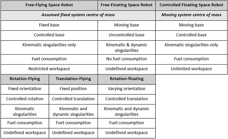
FIGURE 1. Comparison between existing modes of operation for space robot and the CFSR.

2.1 In-Orbit Relative Motion for the CFSR

The literature review reveals that modeling a space robot, which has a controlled spacecraft base, is always performed with respect to an inertial reference frame (Moosavian and Papadopoulos, 2007; Flores-Abad et al., 2014). This is to enable the utilization of Newton’s law of motion to derive the equation of motion of the space robot. Nevertheless, using a space robot for an in-orbit close-proximity approach is described as a three-body problem where it is preferable to reference the motion of the chasing body with respect to the moving and rotating frame of the target body, also known as local vertical local horizontal (LVLH) frame. Then it is necessary to transform the motion in LVLH back to the inertial frame to find the true actuating forces.

In this article, under the assumption that the space robot is operated at a very close proximity to the target (<10 m) and considering a short period (up to 150 s), three frames of reference are selected to derive the equation of motion of the CFSR as shown in Figure 2: the inertial frame ∑_I, the target LVLH frame ∑_T, and the base of the CFSR body frame ∑_B. The idea is to consider the motion of the CFSR in ∑_T as the controllable quantity in the closed-loop control and compute the fictitious forces, originating from the rotating frame ∑_T, as external forces affecting the system. This is to ensure that the true actuating forces and torques are identified in ∑_I.

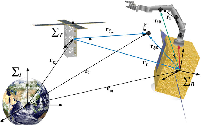
FIGURE 2. Artistic illustration of the reference frames and vectors used in the mathematical model for the CFSR (Seddaoui, 2020).

The motion of the CFSR is described about its overall CoM, referred to here as ξ. Hence, the relative position is defined as the vector between the origin of ∑_T and the CoM ξ, referred to as ${\mathit{r}}_{{\mathit{\xi }}_{\mathit{r}\mathit{e}\mathit{l}}}$. The basic equation of a relative position vector ${\mathit{r}}_{{\mathit{\xi }}_{\mathit{r}\mathit{e}\mathit{l}}}$ in ∑_I is (Curtis, 2013):

where vector ${\mathit{r}}_{\mathit{\xi }}\in {\mathbb{R}}^3$ represents the inertial position vector of the CoM of the space robot ξ, ${\mathit{r}}_{\mathbf{02}}\in {\mathbb{R}}^3$ is the inertial position vector of the target, and ${\mathit{r}}_{{\mathit{\xi }}_{\mathit{r}\mathit{e}\mathit{l}}}\in {\mathbb{R}}^3$ is the relative position vector between ξ and the origin of ∑_T, as shown in Figure 2. The corresponding relative velocity and acceleration vectors in ∑_I are defined as follows (Curtis, 2013):

where $\mathbf{\Omega }\in {\mathbb{R}}^3$ is the angular velocity of the rotating frame ∑_T with respect to ∑_I; ${\mathit{v}}_{\mathit{\xi }}\in {\mathbb{R}}^3$ and ${\mathit{v}}_{\mathbf{02}}\in {\mathbb{R}}^3$ are the velocity vectors of the CoM ξ and the target, respectively; ${\mathit{a}}_{\mathit{\xi }}\in {\mathbb{R}}^3$ and ${\mathit{a}}_{\mathbf{02}}\in {\mathbb{R}}^3$ are the acceleration vectors of the CoM ξ and the target, respectively. In the above equation and thereafter in this article, as it is often customary in the robotics literature, we use the word “vector” to indicate the column matrix of three scalar components of a physical vector in a specific Cartesian triad of axes. Furthermore, we use the symbol of vector cross product in order to indicate the three-by-three skew-symmetric matrix expressing in matricial form the cross product and built with the components of the algebraic vector preceding that symbol.

Eventually, the state vector that will be used in the closed-loop control of the CFSR includes the relative motion between the space robot and the target described by ${\mathit{r}}_{{\mathit{\xi }}_{\mathit{r}\mathit{e}\mathit{l}}}$, ${\dot{r}}_{{\mathit{\xi }}_{\mathit{r}\mathit{e}\mathit{l}}}$ and ${\ddot{\mathit{r}}}_{{\mathit{\xi }}_{\mathit{r}\mathit{e}\mathit{l}}}$. The fictitious velocity and acceleration involved in Eqs 2a, 2b are to be added as extra motion generated from the motion of ∑_T in order to find the true actuating forces and torques in ∑_I. The motion of the space robot’s base has both linear and angular components, as well as the generated interactions between the translational and rotational motion. This is computed through deriving the space robot’s motion about the overall CoM ξ.

3 Spacecraft Motion

The motion of the space robot’s base has both linear and angular components, as well as the generated interactions between the translational and rotational motion. This is computed through deriving the space robot’s motion about the overall CoM ξ.

3.1 The Linear Motion

During close-proximity maneuvers, the relative motion is of interest. Hence, the linear motion of the spacecraft base consists of its own relative motion, as well as that of the arm. It is translated by the relative linear momentum of the system as follows:

where $\mathcal{P}\in {\mathbb{R}}^3$ is the linear momentum of the system; m_i and r_i are, respectively, the mass and the position vector of the ith link of the space robot including the spacecraft base; and M_t is the total mass of the system. Differentiating Eq. 3and substituting Eq. 2b into Eq. 3 gives the equation describing the relative linear motion of the spacecraft base about the CoM (ξ) with respect to ∑_I:

where ${\mathit{F}}_{\mathit{s}\mathit{c}}^{\mathit{I}}\in {\mathbb{R}}^3$ is the force acting on the spacecraft base about ξ in ∑_I. The CoM of the full system ξ is different from the CoM of the base spacecraft. Also, the actuation forces and torques are applied on the spacecraft base rather than ξ. Therefore, in order to derive the equation of the relative linear motion of the spacecraft base, one needs to introduce the motion of ∑_B in ∑_T. Hence, using the equation for the relative velocity and acceleration, as seen in Eqs 2a, 2b, gives the equation for the relative velocity and acceleration ${\dot{r}}_{{\mathit{\xi }}_{\mathit{r}\mathit{e}\mathit{l}}}\in {\mathbb{R}}^3$ and ${\ddot{\mathit{r}}}_{{\mathit{\xi }}_{\mathit{r}\mathit{e}\mathit{l}}}\in {\mathbb{R}}^3$ when considering the motion of ∑_B. In other words, the following represents the expression of the first term of Eqs 2a, 2b when introducing the motion of ∑_B:

where ${\mathit{r}}_{\mathit{T}}\in {\mathbb{R}}^3$ is the relative position vector of the spacecraft base defined as ${\mathit{r}}_{\mathit{T}}={\mathit{r}}_{\mathbf{01}}-{\mathit{r}}_{\mathbf{02}}$, vector ${\mathit{r}}_{\mathit{\xi }\mathit{B}}\in {\mathbb{R}}^3$ represents the relative position vector between ξ and ∑_B, and vector ${\mathit{\omega }}_{\mathit{s}\mathit{c}}\in {\mathbb{R}}^3$ is the angular velocity of the spacecraft base with respect to ∑_T. Multiplying Eq. 5c by the total mass of the system gives the following expression for the linear motion of the spacecraft base in ∑_T, which is function of the spacecraft base’s position vector ${\mathit{r}}_{\mathit{T}}$ instead of the overall CoM’s position vector ${\mathit{r}}_{{\mathit{\xi }}_{\mathit{r}\mathit{e}\mathit{l}}}$, as follows:

where ${\mathit{F}}_{\mathit{s}\mathit{c}}\in {\mathbb{R}}^3$ represents the force acting on the spacecraft base about ξ in ∑_T.

Substituting Eqs 5a, 5b into the last three remaining terms of Eq. 4 gives the following expression for the fictitious forces resulting from the rotation of frame ∑_T:

where ${\mathit{F}}_{\mathit{s}\mathit{c}}^{\mathit{f}\mathit{i}\mathit{c}\mathit{t}}\in {\mathbb{R}}^3$ represents the virtual forces generated from the rotation of the frame ∑_T.

Substituting Eqs 6, 7 into Eq. 4 gives the relative linear motion of the spacecraft base in ∑_I when considering the motion of frame ∑_T. This is expressed as follows:

The first term of Eq. 8 represents the controlled linear motion of the space robot with respect to ∑_T. The second term is related to the rotation of ∑_T, which must be included in the equation of motion to account for the virtual forces that exist only in the rotating frame of reference. Expressing the linear motion of the space robot, represented by Eq. 6, in matrix form gives:

where $\mathbf{E}\in {\mathbb{R}}^{3\times 3}$ is the identity matrix. Eq. 9 describing the relative motion of the spacecraft base is one of the components constituting the equation of the relative motion of the CFSR.

3.2 The Angular Motion

The angular momentum of the multibody space robot about ξ, in terms of the inertia tensor and the angular velocity, is defined, with respect to a frame attached to the CoM of the spacecraft base and that does not rotate with the ∑_B, as follows (see Supplementary Material):

where ${\mathbf{I}}_{\mathbf{\xi }}\in {\mathbb{R}}^{3\times 3}$ and ${\mathbf{I}}_{\mathbf{i}}\in {\mathbb{R}}^{3\times 3}$ are, respectively, the inertia tensors of the full system expressed at the CoM ξ and the ith link of the arm; ω_ξ is the angular velocity about ξ with respect to a frame attached at the origin of ∑_B; and ω_ξB is the angular velocity about ξ with respect to ∑_B.

Let ${\mathbf{I}}_{\mathbf{i}\mathbf{B}}={\sum }_{i=1}^n\left({\mathbf{I}}_{\mathbf{i}}-m_i{[{\mathit{r}}_{\mathit{i}\mathit{B}}]}_{\times }{[{\mathit{r}}_{\mathit{i}\mathit{B}}]}_{\times }\right)$, then Eq. 10 becomes:

Given ω_ξ = ω_sc + ω_ξB, Eq. 10 becomes:

The second and last terms of Eq. 12 are related to the rotation about ξ, generated by the motion of the arm. Differentiating Eq. 12 gives:

As the CFSR is one redundant system, finding the total inertia tensor I_ξ involves two steps: use the parallel axis theorem to express the total inertia matrix of both the spacecraft base and the arm at the origin of ∑_B and then express the result at ξ. The total inertia matrix at the origin of ∑_B is as follows:

Considering the space robot with its overall CoM ξ, which is different from the CoM of the spacecraft base alone, the total inertia tensor of the system at ξ, using the parallel axis theorem, is:

Substituting Eq. 14 into Eq. 15 gives:

It is clear from Eq. 16 that the inertia tensor of the space robot is not constant as it depends on the position of the moving CoM ξ and the moving arm’s links. Hence, the derivatives of the first, second, and third terms of Eq. 13 are given as follows:

The derivatives of the inertia tensors I_ξ and I_iB (see Supplementary Material) still appear in the equation because they are function of position vectors that vary during the motion of the space robot, as seen in Eq. 16.

Substituting 17c and 17d into Eq. 13 gives the equation for the rotational motion of the space robot about ξ as follows:

Eq. 18 describes the rotational dynamics of the space robot about the overall CoM ξ with respect to ξ. Expressing this vector of torques relative to the CoM of the spacecraft base (origin of ∑_B), with respect to ∑_B, requires the following transformation (Curtis, 2013):

Substituting Eqs 8–18 into Eq. 19 and simplifying give:

From Eq. 20, the angular motion of the space robot in ∑_T can be represented in matrix form as follows:

3.3 The Overall Motion of the Spacecraft Base

From Eqs 9–21, the overall equation describing the linear and angular motion of the spacecraft base in ∑_T is:

which can be written in a compact form as follows:

where ${\mathbf{D}}_{\mathbf{v}}\in {\mathbb{R}}^{3\times 3}$, ${\mathbf{D}}_{\mathbf{v}\omega }\in {\mathbb{R}}^{3\times 3}$, ${\mathbf{D}}_{\mathbf{\omega }\mathbf{v}}\in {\mathbb{R}}^{3\times 3}$ and ${\mathbf{D}}_{\mathbf{\omega }}\in {\mathbb{R}}^{3\times 3}$ are mass submatrices related the linear and angular motion of the spacecraft base, as well as the interaction between the linear and angular motion. Vectors ${\mathbf{C}}_{\mathbf{v}}\in {\mathbb{R}}^{3\times 3}$ and ${\mathbf{C}}_{\mathbf{v}\omega }\in {\mathbb{R}}^{3\times 3}$ involve the Coriolis and centrifugal terms originating from the motion of the spacecraft base, and vectors D_ξB and C_ξB are related to the motion of the CoM ξ. The compacted matrix ${\mathbf{D}}_{\mathbf{s}\mathbf{c}}\in {\mathbb{R}}^{6\times 6}$ is related to the linear and angular motion of the spacecraft base, and the compacted vector ${\mathbf{C}}_{\mathbf{s}\mathbf{c}}\in {\mathbb{R}}^{6\times 6}$ involves the Coriolis and centrifugal forces.

4 Manipulator Dynamics

The mathematical model for the dynamics of a terrestrial robotic arm usually involves both the kinetic and the potential energy (Spong and Vidyasagar, 2008). However, space robots operate in a microgravity environment. For this reason, the terms related to the potential energy in the equation of motion are ignored. Hence, only the kinetic energy was used in the Lagrange–Euler method to derive the equation of motion of the robotic arm of the CFSR.

The Lagrange–Euler equation for an n DoF robotic arm is (Spong and Vidyasagar, 2008):

where τ_i is the torque applied the ith joint; L is the Lagrangian function of system L = KE, where KE is the kinetic energy of the arm; θ_i represents the ith joint angle; and ${\dot{\theta }}_i$ is the velocity of the ith joint.

4.1 Kinetic Energy of an n DoF Manipulator

All moving objects have a kinetic energy, and this energy varies according to the mass of the object and the rate of change of the motion (velocity). For a multilink robotic arm, the velocity of each link is represented by the Jacobian matrix and the joint velocity $\dot{\theta }$. The expression for the linear and angular velocities for the ith joint is expressed as follows (Spong and Vidyasagar, 2008):

where ${\mathbf{J}}_{{\mathbf{v}}_{\mathbf{m}\mathbf{i}}}\in {\mathbb{R}}^{3\times n}$ and ${\mathbf{J}}_{{\omega }_{\mathbf{m}\mathbf{i}}}\in {\mathbb{R}}^{3\times n}$ are, respectively, the linear and angular terms of the 6 × n Jacobian matrix of the ith CoM of the arm, and ${\mathbf{R}}_{{\mathbf{L}}_{\mathbf{i}}}\in {\mathbb{R}}^{3\times 3}$ is the rotation matrix of the ith link with respect to ∑_T.

The general equation for the overall kinetic energy for an n DoF manipulator is:

where I_i is the inertia tensor of the ith link about a frame attached at the CoM of the ith link. In order to express the inertia tensor in ∑_T, one has to perform a transformation using the rotation matrix ${\mathbf{R}}_{{\mathbf{L}}_{\mathbf{i}}}$: ${\mathbf{I}}_{\mathbf{i}}^{\mathbf{T}}={\mathbf{R}}_{{\mathbf{L}}_{\mathbf{i}}}{\mathbf{I}}_{\mathbf{i}}{\mathbf{R}}_{{\mathbf{L}}_{\mathbf{i}}}^{\prime }$. Hence, by substituting Eq. 25 into Eq. 26, the expression for the arm’s total kinetic energy is:

Eq. 27 can be written in matrix form:

where ${\mathbf{D}}_{\mathbf{m}}\in {\mathbb{R}}^{n\times n}$ is the symmetric positive definite mass matrix of the robotic manipulator, and it is expressed as:

4.2 The Coriolis and Centrifugal Forces

The joints’ rotational motion results in extra forces known as the Coriolis and centrifugal forces. These forces are computed as follows (Spong and Vidyasagar, 2008):

where c_kj are terms constituting the matrix of Coriolis and centrifugal forces denoted as ${\mathbf{C}}_{\mathbf{m}}\in {\mathbb{R}}^{n\times n}$.

From Eqs 29, 30, the equation describing the linear and angular motion of the arm, the target frame ∑_T is:

5 Jacobian Matrix for the Kinematics of the CFSR

The Jacobian matrix relates the velocity of the end-effector, in the Cartesian space, with the velocity of the space robot, in the configuration space. It describes the kinematics of multibody chain, such as the space robot, at the velocity level. It is expressed as:

The submatrices constituting the Jacobian matrix are defined as follows:

where ${\mathbf{J}}_{{\mathbf{v}}_{\mathbf{s}\mathbf{c}}}\in {\mathbb{R}}^{3\times 6}$ and ${\mathbf{J}}_{{\omega }_{\mathbf{s}\mathbf{c}}}\in {\mathbb{R}}^{3\times 6}$ are, respectively, the linear and rotational components of the Jacobian matrix for the spacecraft base; and ${\mathbf{J}}_{{\mathbf{v}}_{\mathbf{m}}}\in {\mathbb{R}}^{3\times n}$ and ${\mathbf{J}}_{{\omega }_{\mathbf{m}}}\in {\mathbb{R}}^{3\times n}$ are, respectively, the linear and rotational components of the Jacobian matrix for the arm.

The kinematics of a spacecraft can be expressed using either Euler angles or quaternions. Depending on which of these two methods is selected to describe the motion of the space robot, the derivation of the Jacobian matrix varies accordingly. Moreover, when designing a path for the end-effector, the Jacobian matrix related to the end-effector’s position is required, whereas the Jacobian involved in the dynamics is related to the position of the ith CoM of the chain. In the following section, the Jacobian matrix of the CFSR is derived for a potential use with both Euler and quaternions. Also, the end-effector’s velocity, as well as the ith CoM velocity, is described in ∑_T.

5.1 Jacobian Matrix of the End-Effector in ∑_T Using Euler Rate

Deriving the Jacobian matrix of the space robot for use with Euler rate involves several partial derivatives of the rotation matrices as well the spacecraft base’s transformation matrix R_ω defined as follows (Wie, 2008):

5.1.1 The Linear Jacobian of the End-Effector

The linear velocity of the end-effector, in the Cartesian space with respect to ∑_T, is derived using Eq. 2a as follows:

where ${\mathit{r}}_{\mathit{e}\mathit{B}}\in {\mathbb{R}}^3$ is the vector from the origin of ∑_B to the end-effector, as seen in Figure 3 and described as:

where ${\mathit{s}}_{\mathbf{0}}\in {\mathbb{R}}^3$ is the vector from the origin of ∑_B to the first joint of the arm. and ${\mathit{l}}_{\mathit{i}}\in {\mathbb{R}}^3$ is the vector from the ith joint to the (i + 1)^th joint.

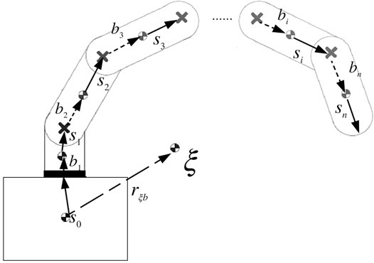
FIGURE 3. Vector representation for the space robot’s physical parameters (Seddaoui, 2020).

The steps of the differentiation of a rotation matrix were presented by Umetani and Yoshida (1989) as follows:

where alpha is the roll angle, beta is pitch angle, and gamma is the yaw angle of the spacecraft base. In addition, phi is the vector of spacecraft base orientation in the target frame.

Using Eq. 36, the linear velocity of the end-effector described by Eq. 34 becomes:

The last term of Eq. 37 involves the body rate ω_sc which can be a function of Euler rate and R_ω using Eq. 33. The linear velocity described by Eq. 37 then becomes:

From Eq. 38, the linear Jacobian submatrices for both the spacecraft base and the arm are:

where $\mathbf{E}\in {\mathbb{R}}^{3\times 3}$, ${\mathbf{J}}_{{\mathbf{v}}_{\mathbf{s}\mathbf{c}}}^{″}(1),{\mathbf{J}}_{{\mathbf{v}}_{\mathbf{s}\mathbf{c}}}^{″}(2),{\mathbf{J}}_{{\mathbf{v}}_{\mathbf{s}\mathbf{c}}}^{″}(3)\in {\mathbb{R}}^3$, ${\mathbf{J}}_{{\mathbf{v}}_{\mathbf{m}}}^{″}(j)\in {\mathbb{R}}^3$ and e₁, e₂, e₃ are unit vectors.

5.1.2 The Rotational Jacobian of the End-Effector

The angular velocity of the end-effector can be expressed as:

where ${\mathit{\omega }}_{\mathit{e}}\in {\mathbb{R}}^3$ is the angular velocity of the end-effector in ∑_T, ${\mathit{\omega }}_{\mathit{e}\mathit{B}}\in {\mathbb{R}}^3$ is the angular velocity of the end-effector in ∑_B, and ${\mathit{\omega }}_{\mathit{s}\mathit{c}}\in {\mathbb{R}}^3$ is the angular velocity of the spacecraft base in ∑_T.

Using Eqs 33–40, ω_e becomes:

From Eq. 41, the rotational Jacobian submatrices for both the spacecraft base and the arm are:

where $\mathbf{0}\in {\mathbb{R}}^{3\times 3}{\mathbf{J}}_{{\omega }_{\mathbf{s}\mathbf{c}}}^{″}(j)\in {\mathbb{R}}^3$ and ${\mathbf{J}}_{{\omega }_{\mathbf{m}}}^{″}(j)\in {\mathbb{R}}^3$ and e₁, e₂ and e₃ are unit vectors.

5.1.3 The Full Jacobian Translating the Velocities of the End-Effector

From Eqs 39–42, the overall Jacobian matrix for the space robot is as follows:

5.2 Jacobian Matrix of the ith CoM in ∑_T Using Euler Rate

The Jacobian described by Eq. 43 is used to find the position of the end-effector in the Cartesian space, given a configuration or the inverse procedure for path planning. However, the matrices ${\mathbf{J}}_{{\mathbf{v}}_{{\mathbf{m}}_{\mathbf{i}}}}$ and ${\mathbf{J}}_{{\omega }_{{\mathbf{m}}_{\mathbf{i}}}}$ of Eq. 29 relate to the velocity of the CoM of the ith link with the velocities in the configuration space. For this reason, the equations for ${\mathbf{J}}_{{\mathbf{v}}_{{\mathbf{m}}_{\mathbf{i}}}}$ and ${\mathbf{J}}_{{\omega }_{{\mathbf{m}}_{\mathbf{i}}}}$ in Eq. 29 are different from those for ${\mathbf{J}}_{{\mathbf{v}}_{\mathbf{m}}}$ and ${\mathbf{J}}_{{\omega }_{\mathbf{m}}}$ in Eqs 39–42.

5.2.1 The Linear Jacobian of the ith CoM

Using Eq. 2a, the linear velocity of the ith CoM, with respect to ∑_T, is determined as follows:

where r_iB is the vector from the origin of ∑_B to the ith CoM, as seen in Figure 3. It is represented by the following equation:

where ${\mathit{b}}_{\mathit{i}}\in {\mathbb{R}}^3$ is the vector from the ith joint to the CoM of the ith link, and ${\mathit{s}}_{\mathit{i}-\mathit{1}}\in {\mathbb{R}}^3$ is the vector from the CoM of the (i − 1)^th link to the ith joint as shown in Figure 3.

Differentiating Eq. 45 and using the derivatives of the rotation matrix in Eq. 36 give:

References

Artigas, J., De Stefano, M., Rackl, W., Lampariello, R., Brunner, B., Bertleff, W., et al. (2015). “The Oos-Sim: An On-Ground Simulation Facility for On-Orbit Servicing Robotic Operations,” in IEEE International Conference on Robotics and Automation (ICRA). Seattle, 26–30. doi:10.1109/icra.2015.7139588
[Dataset] Satellite Catapult Applications, Fair-Space and Astroscale (2021). A $1bn uk Opportunity for In-Orbit Services. Available at: https://sa.catapult.org.uk/news/in-orbit-servicing-capability (Last Accessed June 13, 2021).
Dubowsky, S., and Papadopoulos, E. (1993). The Kinematics, Dynamics, and Control of Free-Flying and Free-Floating Space Robotic Systems. IEEE Trans. Robot. Automat. 9, 531–543. doi:10.1109/70.258046
Flores-Abad, A., Ma, O., Pham, K., and Ulrich, S. (2014). A Review of Space Robotics Technologies for On-Orbit Servicing. Prog. Aerospace Sci. 68, 1–26. doi:10.1016/j.paerosci.2014.03.002
Friend, R. B. (2008). “Orbital Express Program Summary and mission Overview,” in SPIE Defense and Security Symposium (Orlando, FL: International Society for Optics and Photonics), 695–803. doi:10.1117/12.783792
Guang, Z., Heming, Z., and Liang, B. (2018). Attitude Dynamics of Spacecraft with Time-Varying Inertia during On-Orbit Refueling. J. Guidance, Control Dyn., 1–11. doi:10.2514/1.g003474
Jackson, L., Saaj, C. M., Seddaoui, A., Whiting, C., Eckersley, S., and Hadfield, S. (2020). Downsizing an Orbital Space Robot: A Dynamic System Based Evaluation. Adv. Space Res. 65, 2247–2262. doi:10.1016/j.asr.2020.03.004
Jaekel, S., Lampariello, R., Panin, G., Sagardia, M., Brunner, B., Porges, O., et al. (2015). “Robotic Capture and De-orbit of a Heavy, Uncooperative and Tumbling Target in Low Earth Orbit,” in 13th Symposium on Advanced Space Technologies in Robotics and Automation (Noordwijk, Netherlands: ASTRA), 11–13.
Lee, N., Backes, P., Burdick, J., Pellegrino, S., Fuller, C., Hogstrom, K., et al. (2016). Architecture for In-Space Robotic Assembly of a Modular Space Telescope. J. Astronomical Telescopes, Instr. Syst. 2, 041207. doi:10.1117/1.jatis.2.4.041207
Li, W.-J., Cheng, D.-Y., Liu, X.-G., Wang, Y.-B., Shi, W.-H., Tang, Z.-X., et al. (2019). On-orbit Service (Oos) of Spacecraft: A Review of Engineering Developments. Prog. Aerospace Sci. 108, 32–120. doi:10.1016/j.paerosci.2019.01.004
Longman, R. W., Lindbergt, R. E., and Zedd, M. F. (1987). Satellite-Mounted Robot Manipulators - New Kinematics and Reaction Moment Compensation. Int. J. Robotics Res. 6, 87–103. doi:10.1177/027836498700600306
Medina, A., Tomassini, A., Suatoni, M., Avilés, M., Solway, N., Coxhill, I., et al. (2017). Towards a Standardized Grasping and Refuelling On-Orbit Servicing for Geo Spacecraft. Acta Astronautica 134, 1–10. doi:10.1016/j.actaastro.2017.01.022
Menon, C., Busolo, S., Cocuzza, S., Aboudan, A., Bulgarelli, A., Bettanini, C., et al. (2007). Issues and Solutions for Testing Free-Flying Robots. Acta Astronautica 60, 957–965. doi:10.1016/j.actaastro.2006.11.014
Moosavian, S. A. A., and Papadopoulos, E. (2007). Free-flying Robots in Space: an Overview of Dynamics Modeling, Planning and Control. Robotica 25. doi:10.1017/s0263574707003438
Nair, M. H., Saaj, C. M., Esfahani, A. G., Nanjangud, A., Eckersley, S., and Bianco, P. (2020). “In-space Robotic Assembly and Servicing of High-Value Infrastructure,” in Proc. International Astronautical Congress. Cyberspace Edition (Dubai: IAC2020).
Oda, M., Kibe, K., and Yamagata, F. (1996). “Ets-vii, Space Robot In-Orbit experiment Satellite,” in Proc. 1996 IEEE International Conference on Robotics and Automation, Minnesota, April 22-28, 739–744.
Papadopoulos, E., and Dubowsky, S. (1991). “Coordinated Manipulator/spacecraft Motion Control for Space Robotic Systems,” in IEEE International Conference on Robotics and Automation, Sacramento, April, 9–11, 1696–1701.
Papadopoulos, E., and Dubowsky, S. (1993). Dynamic Singularities in Free-Floating Space Manipulators. J. Dynamic Syst. Meas. Control 115, 44–52. doi:10.1115/1.2897406
Reed, B. B., Smith, R. C., Naasz, B., Pellegrino, J., and Bacon, C. (2016). “The Restore-L Servicing mission,” in AIAA Space Conference, Long Beach California, September, 13–16. doi:10.2514/6.2016-5478
Romano, M. (2021). Space Robotics. Cham: Springer International Publishing, 2090–2097. doi:10.1007/978-3-030-44184-5_100035
Seddaoui, A. (2020). Precise Motion Control of a Space Robot for In-Orbit Close Proximity Manoeuvres. Ph.D. thesis (Guildford, UK: University of Surrey).
Seddaoui, A., and Saaj, C. M. (2021). Collision-free Optimal Trajectory Generation for a Space Robot Using Genetic Algorithm. Acta Astronautica 179, 311–321. doi:10.1016/j.actaastro.2020.11.001
Seddaoui, A., and Saaj, C. M. (2019). Combined Nonlinear H∞ Controller for a Controlled-Floating Space Robot. J. Guidance, Control Dyn. 42, 1878–1885. doi:10.2514/1.g003811
Seddaoui, A., Saaj, C. M., and Eckersley, S. (2019). “Adaptive H Infinity Controller for Precise Manoeuvring of a Space Robot,” in Proc. IEEE International Conference on Robotics and Automation, Montreal, May, 20–24 (Reston, VA: ICRA).
Spong, M. W., and Vidyasagar, M. (2008). Robot Dynamics and Control. United States: John Wiley & Sons.
Taylor, B., Aglietti, G., Fellowes, S., Ainley, S., Salmon, T., Retat, I., et al. (2018). “Remove Debris mission, from Concept to Orbit,” in 32nd Annual AIAA/USU Conference on Small Satellites, Utah, August, 4–9.
Umetani, Y., and Yoshida, K. (1989). Resolved Motion Rate Control of Space Manipulators with Generalized Jacobian Matrix. IEEE Trans. Robot. Automat. 5, 303–314. doi:10.1109/70.34766
Virgili-Llop, J., Drew, J. V., Zappulla, R., and Romano, M. (2017). Laboratory Experiments of Resident Space Object Capture by a Spacecraft-Manipulator System. Aerospace Sci. Technology 71, 530–545. doi:10.1016/j.ast.2017.09.043
Virgili-Llop, J., and Romano, M. (2019). Simultaneous Capture and Detumble of a Resident Space Object by a Free-Flying Spacecraft-Manipulator System. Front. Robot. AI 6, 14. doi:10.3389/frobt.2019.00014
Virgili-Llop, J., Zagaris, C., Zappulla, R., Bradstreet, A., and Romano, M. (2019). A Convex-Programming-Based Guidance Algorithm to Capture a Tumbling Object on Orbit Using a Spacecraft Equipped with a Robotic Manipulator. Int. J. Robotics Res. 38, 40–72. doi:10.1177/0278364918804660
Whittaker, W., Urmson, C., Staritz, P., Kennedy, B., and Ambrose, R. (2000). “Robotics for Assembly, Inspection, and Maintenance of Space Macrofacilities,” in Proc. AIAA Space Conference and Exposition.
Wie, B. (2008). Space Vehicle Dynamics and Control. American Institute of Aeronautics and Astronautics.
Wilde, M., Kwok Choon, S., Grompone, A., and Romano, M. (2018). Equations of Motion of Free-Floating Spacecraft-Manipulator Systems: An Engineer's Tutorial. Front. Robot AI 5, 41. doi:10.3389/frobt.2018.00041
Wilde, M., Harder, J., and Stoll, E. (2019). Editorial: On-Orbit Servicing and Active Debris Removal: Enabling a Paradigm Shift in Spaceflight. Front. Robot. AI 6, 136. doi:10.3389/frobt.2019.00136
Xu, Y. (2021). Adaptive Attitude-Tracking Control of Spacecraft Considering On-Orbit Refuelling. Trans. Inst. Meas. Control. 43, 1298–1309. doi:10.1177/0142331220973132
Xu, Y., and Kanade, T. (1992). Space Robotics: Dynamics and Control, 188. Springer Science & Business Media.
Xu, Y. (1993). “The Measure of Dynamic Coupling of Space Robot Systems,” in IEEE International Conference on Robotics and Automation, Atlanta, May, 2–6.
Yoshida, K., and Abiko, S. (2002). “Inertia Parameter Identification for a Free-Flying Space Robot,” in AIAA Guidance, Navigation, and Control Conference and Exhibit, California, August, 5–8. doi:10.2514/6.2002-4568
Keywords: space robot, free-flying, free-floating, controlled-floating, pose control, dynamic modeling
Citation: Seddaoui A, Saaj CM and Nair MH (2021) Modeling a Controlled-Floating Space Robot for In-Space Services: A Beginner’s Tutorial. Front. Robot. AI 8:725333. doi: 10.3389/frobt.2021.725333
Received: 15 June 2021; Accepted: 02 November 2021;
Published: 24 December 2021.
Edited by:
Marcello Romano, Naval Postgraduate School, United StatesReviewed by:
Simone Chesi, Maxar Technologies, United StatesJennifer Hudson, Naval Postgraduate School, United States
Fabio Curti, Sapienza University of Rome, Italy
Copyright © 2021 Seddaoui, Saaj and Nair. This is an open-access article distributed under the terms of the Creative Commons Attribution License (CC BY). The use, distribution or reproduction in other forums is permitted, provided the original author(s) and the copyright owner(s) are credited and that the original publication in this journal is cited, in accordance with accepted academic practice. No use, distribution or reproduction is permitted which does not comply with these terms.
*Correspondence: Chakravarthini Mini Saaj , MSaaj@lincoln.ac.uk