If you were to ask one-hundred shooting coaches “What’s the most important aspect to making a jump shot?” you will probably get at least fifty different responses. Answers may range from detailed such as the finger mechanics of the release or “shooting axis,” to broad, holistic responses such as “Find your repeatable comfort zone at game speed.” On the analytics end of the spectrum, the analysis is seemingly straightforward: put the ball on a projectile trajectory with the appropriate initial values to ensure the ball goes through the hoop.
Go ahead and eye roll. I’ll wait.
While this sounds like there should be a “yeah, but” type response, let’s instead think through the analytic process in real life. When we talk about the components of a field goal attempt, we may talk about items such as lift, squaring, and follow through. These are those initial values mentioned above. Traditionally, projectile motion follows a three dimensional parabolic-type path defined by initial motion of the projectile and the acceleration forces applied to the ball while in flight. In essence, we identify squaring as setting the rotational angle of the jump shot and lift as the upward motion of the ball. From there, follow through can be seen as setting the drag of the ball through rotation, effectively impacting the time of arrival for the basketball to its descent.
It’s at this point, we can start talking about the physical process of a jump shot from an analytic perspective. By modeling the flight of a basketball, we are able to quantify the components associated with life, squaring, and follow-through in such as way that we can begin answering much more impactful questions; such as “how do close outs affect a particular player?” or “What’s the effect of receiving a ball in a catch-and-shoot on the release of a jump shot?” or “How does an escape dribble change the release of a jump shot?”
This allows us to throw away generic “your hand needs to be here” approaches and take individualized looks at each player to maximize vitamin time when it comes to developing a jump shot touch at game speed. Candidly, it would also allow us to better understand why players like Larry bird or Reggie Miller could have “poor shooting form” but yet be such prolific shooters.*
To do this, we rely on approximating curves, but not in a “let’s hammer a regression and cross our fingers!” sense. Instead, we apply a more robust methodology by injecting the physical process of a jump shot and calibrate the physical model through data assimilation.
Three Dimensional Motion
To keep this modeling technique relatively simple, let’s focus on only the projectile motion of a jump shot. To illustrate, let’s start with a simple example. Suppose we take a jump shot from a particular location, say (x,y) and release the ball at a height, z. Further suppose the jump shot is converted by hitting center-of-cylinder, with total travel time taking exactly T seconds from release to basket. What is the initial velocity vector of the jump shot?
To solve this using only (x,y,z) coordinates of the basketball, we first make an assumption about the flight path of the basketball. This is traditionally parabolic in nature and is additionally governed by external acceleration forces such as gravity. Those equations are given by
where x(t) denotes the baseline location of the basketball at time t, y(t) denotes the sideline location of the basketball at time t, and z(t) denotes the height of the basketball at time t.
If we make a basic assumption that only gravity affects the basketball during flight, then we can assume a constant acceleration vector of [0, 0, -32.185]. Here, we are operating in feet as opposed to meters as many fans are accustomed to the 50′ x 94′ court. We also place a negative value as gravity pulls the ball back down to the court. The x- and y-values having zero acceleration indicates that there are no external forces pulling the ball across the court. This may be not true in practice as there may be drafts from open court plans and friction generated by the rotation of the ball through the air. Here, we assume that is noise in the system.
This now reduces our physical model to
This means that if we look at a particular jump shot, we can “solve” the equation to extract out the velocity vector, which indicates squaring and lifting:

Therefore, if we were to take a midrange jump shot from just outside the elbow, and make the basket, we obtain the equation for the required initial condition to make the basket from the above formula, which is now a function of time. Therefore, if we wanted to model a Jordan jump shot, we could look at time of flight, release point, and landing spot.
Using the parameterization above, the 3-D image would look like this:
However, if we looked at a Purvis Short style jump shot, we would identify a higher arc as the value of T increases:
In essence, we can take a couple points on the trajectory and recover the parabolic trajectory of the field goal attempt.
Explicitly, in the Michael Jordan and Purvis Short examples above, all we did was take two “routine” uncontested jump shot attempts, rounded to the nearest second, and made the assumption that both attempts were released at the same location, at the same height, with the same end location. For the illustrations above, these values are start = [35.89, 27.88, 9] and finish = [25.15, 41.57, 10], with T = 1.0 versus T = 2.0. For reference, from the sample of attempts, Jordan’s time of flight from roughly that region was 1.2 seconds while Short’s was roughly 1.8 seconds.
Using the illustration values above, we find that the direction of release for Jordan is [-0.4402, 0.5614, 0.7008] with a speed of release at 24.39 feet per second. Similarly for Short, we have a direction of release at [-0.1587, 0.2024, 0.9664] with a speed of release at 33.82 feet per second.
Now, if we are to accept this crude method for estimating shot release, we can now look at the distribution of shot release vectors and build ourselves a statistical test of hypotheses using random effects and the vector response. Hint: Wait for part three of this series…
The problem here is that this is indeed a crude method we outlined. Suppose there is 0.2 seconds of error in the timing of the arrival of the basketball, as we injected into both the Jordan and Short attempts above. With a slight adjustment of 0.2 seconds, we see that Jordan’s release changes from [-0.4402, 0.5614, 0.7008] with 24.39 to [-0.3605, 0.4597, 0.8116] with 24.82. This could be the difference in seeing a true effect on a shot attempt or just random noise in the system. Fortunately, the noise is not as significant. With tracking systems such as Second Spectrum, we are able to reduce this sampling error down to approximately .04 seconds.
However, we are still forced to deal with error in the system.
Data Assimilation
As a field goal attempt follows a physical process such as projectile motion, we have a process equation that defines a sequence of points generated from an initial state. This process equation can be viewed as deterministic, which indicates there is no noise in the process, that is: the process perfectly describes the physical phenomenon; or it can be viewed as stochastic, which indicates there are missing components of the model and this introduces errors between the mathematical formulation and the real life phenomenon. Similarly, we have a measurement equation that defines a method for observing points about the physical process. This too introduces error into the system as our measuring tools are noisy.
Therefore, the aim of the statistical problem is to account for both process noise and measurement noise in such a a way that we can best approximate the physical process of interest. Think of this as “curve fitting” by using the physical system as a “penalty.” By viewing it this way, this statistical methodology, called data assimilation, is viewed as Bayesian curve fitting problem traditionally called optimal statistical interpolation. The most commonly known, yet lackluster for physical systems, method of data assimilation is the Kalman Filter. While the Kalman Filter is a nice application of smoothing, it requires significant tuning of the process and measurement covariance matrices; which may be sensitive to randomness within the initial conditions of the physical process. Therefore, we look at variational methods such as the 4D-Var and the Ensemble Kalman Filter models.
4D-Var is a methodology that observes physical process points within a window of time called the assimilation window and performs a fit of the cost function
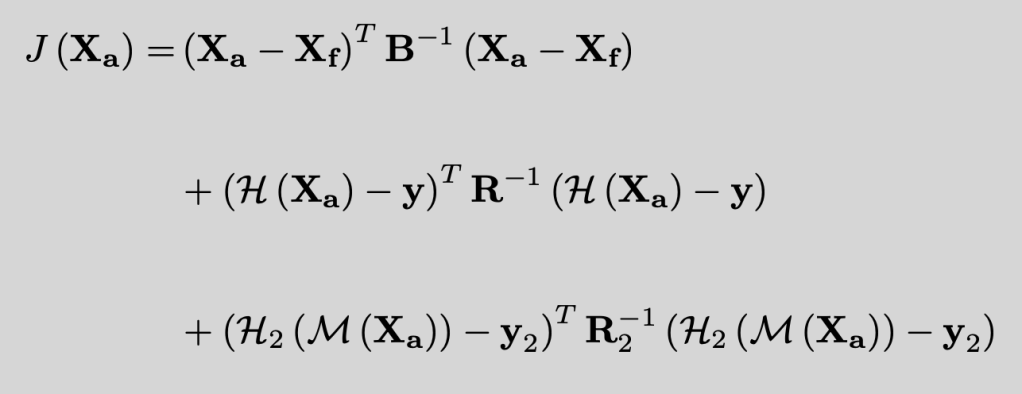
where Xa is the analysis of the system, Xf is the forecast of the system, H is the measurement function of the process, M is the forecast function between two time points within the system, and y is the observation of the system. Here, analysis looks at the difference between the state of a physical system and its associated forecast. Let’s tether these concepts to the jump shot example.
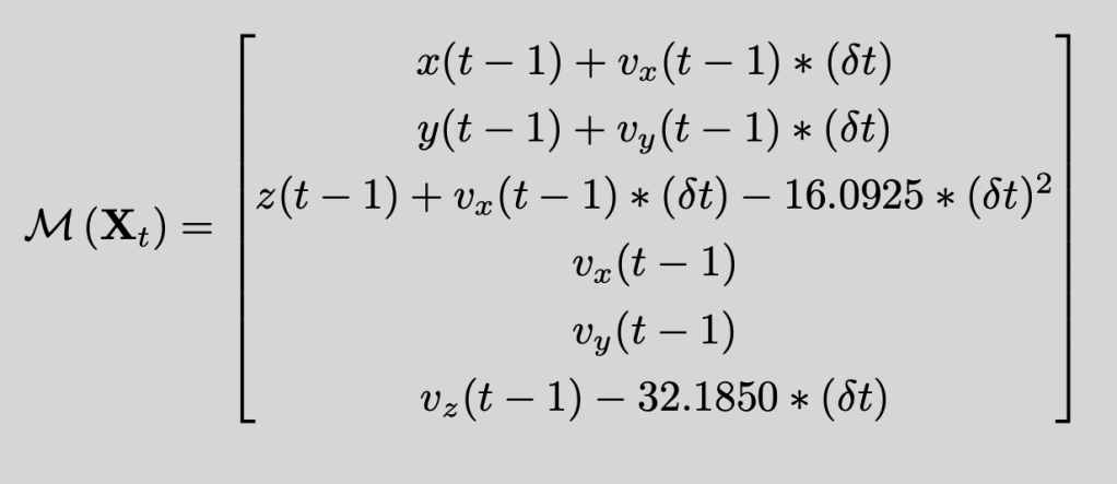
Using a second spectrum system, we obtain (x,y,z) coordinates of the basketball. We already know the process, M. This is the mechanical equation given by
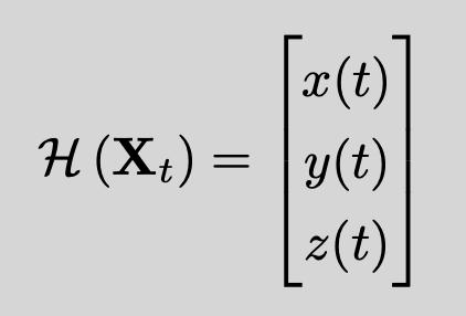
The measurement function is quite obvious. It is the identity function. That is, we obtain states of the system using (x,y,z) coordinates and the second spectrum camera system reports observations in the (x,y,z) coordinate space. On the second spectrum end, however, they would see pixel locations as their state of the system and the measurement function would be a conversion from (x,y,z) to (pixel, camera).
Therefore, since we have M and H defined, we can see that the states, X are just positions in the state of the system: Xf is the forecast using the mechanical process. The values y are observations from the second spectrum camera system. Xa is the optimal state of the system defined by the data observations and the physical process. This is what we are trying to identify!!!
Finally, the covariance matrices are given by B and R. These are estimated within the optimization stages.
The power of a 4D-Variational model is through its optimization scheme. Taking a look at the cost function, you’d be hard-pressed to believe that it is indeed a Bayesian problem. It not only is a Bayesian methodology, but a solution to the system will be a Best Linear Unbiased Estimator (BLUE) of the actual flight path of the ball! The devil is in the details of the optimization, which leverages an “inner” and “outer” loop as the optimization both runs “forward” and “backward” in time using the adjoint of the physical process.
Example: Serge Ibaka
Let’s look at an example of a particular player: Serge Ibaka. The reason we select him is due to his dramatic shift from being a prototypical power-forward to a perimeter hawk over the span of effectively one year. If we take a sample of jump shots from Serge Ibaka’s career, we obtain the following noisy set of jump shots:
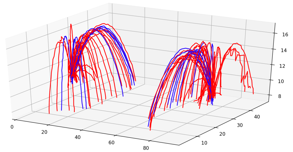
Portions that look like “bunnies” are rebounds that slipped through the filtration process.
Here we indeed see the parabolic nature of the jump shot for the sample. Furthermore, we also indeed see the noisy trajectories for each attempt! Those fluctuations, for the most part, are effectively 6-12 inches of measurement error. Some attempts are fairly bad, such as the pair of corner three attempts on the right-hand-side of the plot.
Here, we mark made attempts as blue and missed attempts as red. Visually, we can start to make assertions about the trajectory of the ball against being a “make’ or a “miss.” The blue trajectories are tighter, suggesting they are following the optimal path. The red trajectories are more varied, showing deviation from optimal path would suggest a miss.
That said, a player cannot control a trajectory mid-flight. It all comes from the release. Therefore, we appeal back to approximating the curve and leverage the physical process through data assimilation to recover the components of the player’s action taken: initial values of the physical system.
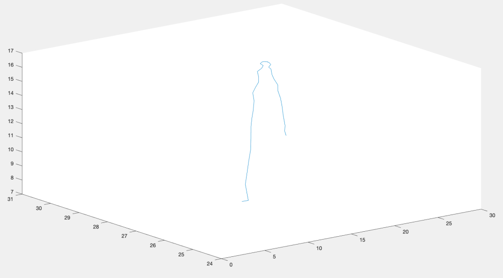
Let’s isolate one made attempt:
We can apply linear regression to get a beautiful looking curve, but the error associated with the high curvature components will dominate the regression and actually bias the result. More specifically, the quantity we need, release vector, will suffer from unintended noise from the statistical calculation. More importantly, the laws of physics would be violated in favor of such a regression.
Instead, we apply the 4D-Var methodology and minimize that ugly looking cost function from above:

Since the assimilation window is over the arc of the field goal attempt, we differentiate with respect to all states, in this case 39 samples, of trajectory. In doing this, we obtain the constraints
The first equation is ensuring that the forecasted state matched the the actual state of the system as closely as possible. The second equation is the loss function associated across all fits simultaneously. This approach leads to the adjoint method of optimization; which can be thought of as being akin to backpropagation in neural networks.
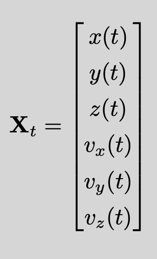
Now, let’s be explicit on the state of the system. Recall that the initial values are release point and velocity vector. This means the state of the system is not the (x,y,z) coordinates but rather:
Our forecast function is then:
And the measurement function is simply:
By using an assumption is effectively 6 inches of measurement and process error, we use diagonal representations for B and R and perform the above optimization. The result for the above given field goal attempt is then
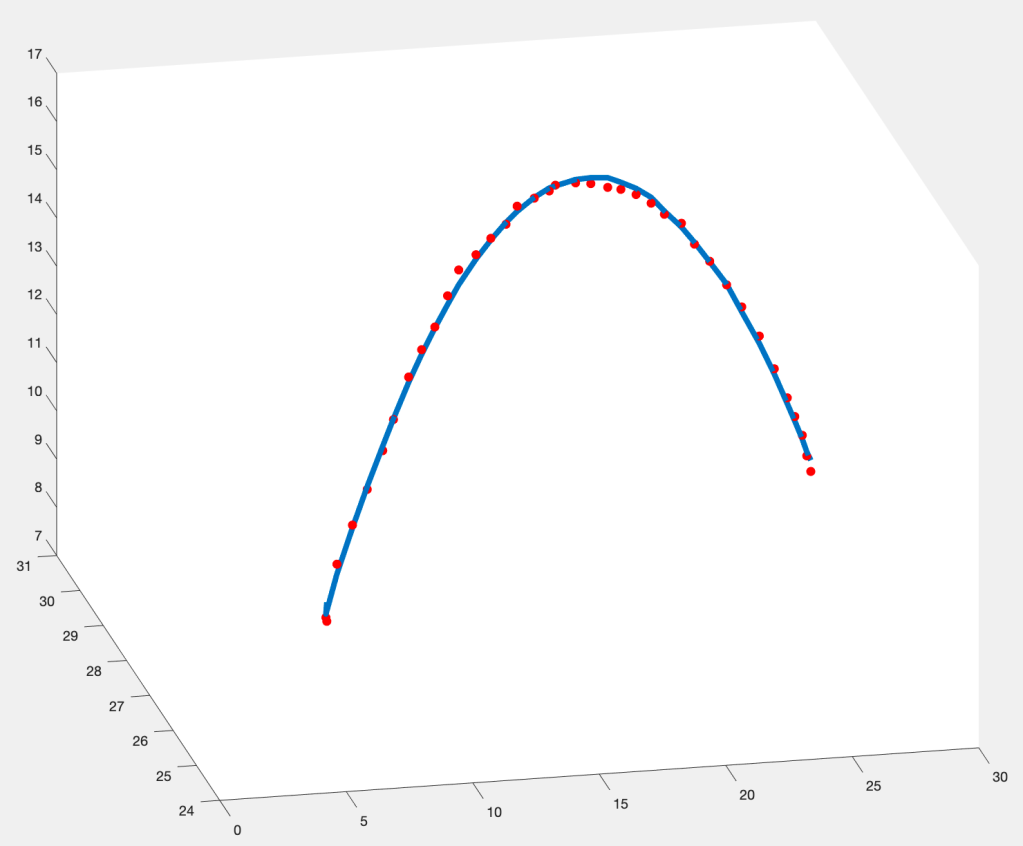
We see the much smoother estimate of the shot arc. More importantly, the shot attempt is following the laws of physics much more than a regression model. Thirdly, we are able to crack open the state of the system and look at the velocity component.
In this case, the release vector is [-0.5264, -0.1268, 0.8407] with a speed of 30.72 feet per second. Don’t feel compelled to look back at the Jordan/Short examples; as those are midrange jump shots. Similarly, it should make sense for a shot taken from further depth requires more “strength” on the shot.
But at this moment, we are able to quantify a shooter’s touch on the ball through the use of a physical system through data assimilation. While this is a neat technique, this is by no means an end to the analytic process.
In part three, we will see how questions of interest can be turned into statistical investigations. From the shooting coach perspective, we can begin quantifying how a player adapts to a vitamin adjustment. From a coaching standpoint, we can look at the effect of a close-out on the actual mechanics of a field goal attempt, as opposed to generating a proxy make/miss response which is typically too noisy.
And in the end, we can begin to remove ourselves from the “take 10,000 shots” thought and look at “strategic training” to optimize time in gym; as well as identify player-specific traits that can either be improved or exploited in game-situation.







Absolutely amazing analysis. Thank you for this blog and everything you provide publicly.
LikeLike