How to Create a Custom 2D Physics Engine: Oriented Rigid Bodies

So far, we've covered impulse resolution, the core architecture, and friction. In this, the final tutorial in this series, we'll go over a very interesting topic: orientation.

In this article we will discuss the following topics:

Rotation math
Oriented shapes
Collision detection
Collision resolution

I highly recommended reading up on the previous three articles in the series before attempting to tackle this one. Much of the key information in the previous articles are prerequisites to rest of this article.

Sample Code

I've created a small sample engine in C++, and I recommend that you browse and refer to the source code throughout the reading of this article, as many practical implementation details could not fit into the article itself.

This GitHub repo contains the sample engine itself, along with a Visual Studio 2010 project. GitHub allows you to view the source without needing to download the source itself, for convenience.

Orientation Math

The math involving rotations in 2D is quite simple, although a mastery of the subject will be required to create anything of value in a physics engine. Newton's second law states:

\[ Equation \: 1:\\
F = ma\]

There is a similar equation that relates specifically angular force and angular acceleration. However, before these equations can be shown, a quick description of the cross product in 2D is required.

Cross Product

The cross product in 3D is a well known operation. However, the cross product in 2D can be quite confusing, as there isn't really a solid geometric interpretation.

The 2D cross product, unlike the 3D version, does not return a vector but a scalar. This scalar value actually represents the magnitude of the orthogonal vector along the z-axis, if the cross product were to actually be performed in 3D. In a way, the 2D cross product is just a simplified version of the 3D cross product, as it is an extension of 3D vector math.

If this is confusing, do not worry: a thorough understanding of the 2D cross product is not all that necessary. Just know exactly how to perform the operation, and know that the order of operations is important: \(a \times b\) is not the same as \(b \times a\). This article will make heavy use of the cross product in order to transform angular velocity into linear velocity.

Knowing how to perform the cross product in 2D is very important, however. Two vectors can be crossed, a scalar can be crossed with a vector, and a vector can be crossed with a scalar. Here are the operations:


// Two crossed vectors return a scalar
float CrossProduct( const Vec2& a, const Vec2& b )
{
  return a.x * b.y - a.y * b.x;
}

// More exotic (but necessary) forms of the cross product
// with a vector a and scalar s, both returning a vector
Vec2 CrossProduct( const Vec2& a, float s )
{
  return Vec2( s * a.y, -s * a.x );
}

Vec2 CrossProduct( float s, const Vec2& a )
{
  return Vec2( -s * a.y, s * a.x );
}

Torque and Angular Velocity

As we all should know from the previous articles, this equation represents a relationship between the force acting upon a body with that body's mass and acceleration. There is an analog for rotation:

\[ Equation \: 2:\\
T = r \: \times \: \omega\]

\(T\) stands for torque. Torque is rotation force.

\(r\) is a vector from the center of mass (COM) to a particular point on an object. \(r\) can be thought of as referring to a "radius" from COM to a point. Every single unique point on an object will require a different \(r\) value to be represented in Equation 2.

\(\omega\) is called "omega", and refers to rotational velocity. This relationship will be used to integrate angular velocity of a rigid body.

It is important to understand that linear velocity is the velocity of the COM of a rigid body. In the previous article, all objects had no rotational components, so the linear velocity of the COM was the same velocity for all points on a body. When orientation is introduced, points farther away from the COM rotate faster than those near the COM. This means we need a new equation to find the velocity of a point on a body, since bodies can now spin and translate at the same time.

Use the following equation to understand the relationship between a point on a body and the velocity of that point:

\[ Equation \: 3:\\
\omega = r \: \times v \]

\(v\) represents linear velocity. To transform linear velocity into angular velocity, cross the \(r\) radius with \(v\).

Similarly, we can rearrange Equation 3 to form another version:

\[ Equation \: 4:\\
v = \omega \: \times r \]

The equations from the last section are quite powerful only if rigid bodies have uniform density. Non-uniform density makes the math involved in calculating anything required the rotation and behavior of a rigid body much too complicated. Furthermore, if the point representing a rigid body is not at the COM, then the calculations regarding \(r\) are going to be entirely wonky.

Inertia

In two dimensions an object rotates about the imaginary z-axis. This rotation can be quite difficult depending on how much mass an object has, and how far away from the COM the object's mass is. A circle with mass equal to a long thin rod will be easier to rotate than the rod. This "difficulty to rotate" factor can be thought of as the moment of inertia of an object.

In a sense, inertia is the rotational mass of an object. The more inertia something has, the harder it is to get it spinning.

Knowing this, one could store the inertia of an object within the body as the same format as mass. It would wise to also store the inverse of this inertia value, being careful not to perform a division by zero. Please see the previous articles in this series for more information on mass and inverse mass.

Integration

Each rigid body will require a few more fields to store rotational information. Here's a quick example of a structure to hold some additional data:


struct RigidBody
{
  Shape *shape

  // Linear components
  Vec2 position
  Vec2 velocity
  float acceleration

  // Angular components
  float orientation // radians
  float angularVelocity
  float torque
};

Integrating the angular velocity and orientation of a body are very similar to the integration of velocity and acceleration. Here is a quick code sample to show how it's done (note: details about integration were covered in a previous article):


const Vec2 gravity( 0, -10.0f )
velocity += force * (1.0f / mass + gravity) * dt
angularVelocity += torque * (1.0f / momentOfInertia) * dt
position += velocity * dt
orient += angularVelocity * dt

With the small amount of information presented so far, you should be able to start rotating various things on the screen without any trouble. With just a few lines of code, something rather impressive can be constructed, perhaps by tossing a shape into the air while it rotates about the COM as gravity pulls it downward to form an arced path of travel.

`Mat22`

Orientation should be stored as a single radian value, as seen above, though often times the use of a small rotation matrix can be a much better choice for certain shapes.

A great example is the Oriented Bounding Box (OBB). The OBB consists of a width and height extent, both of which can be represented by vectors. These two extent vectors can then be rotated by a two-by-two rotation matrix to represent the axes of an OBB.

I suggest the creation of a Mat22 matrix class to be added to whatever math library you are using. I myself use a small custom math library which is packaged in the open source demo. Here is an example of what such an object may look like:


struct Mat22
{
  union
  {
    struct
    {
      float m00, m01
      float m10, m11;
    };

    struct
    {
      Vec2 xCol;
      Vec2 yCol;
    };
  };
};

Some useful operations include: construction from angle, construction from column vectors, transpose, multiply with Vec2, multiply with another Mat22, absolute value.

The last useful function is to be able to retrieve either the x or y column from a vector. The column function would look something like:

1
2	Mat22 m( PI / 2.0f );
3	Vec2 r = m.ColX( ); // retrieve the x axis column

This technique is useful for retrieving a unit vector along the an axis of rotation, either the x or y axis. Additionally, a two-by-two matrix can be constructed from two orthogonal unit vectors, as each vector can be directly inserted into the rows. Although this construction method is a bit uncommon for 2D physics engines, it can still be very useful to understand how rotations and matrices work in general.

This constructor might look something like:


Mat22::Mat22( const Vec2& x, const Vec2& y )
{
  m00 = x.x;
  m01 = x.y;
  m01 = y.x;
  m11 = y.y;
}

// or

Mat22::Mat22( const Vec2& x, const Vec2& y )
{
  xCol = x;
  yCol = y;
}

Since the most important operation of a rotation matrix is to perform rotations based off of an angle, it's important to be able to construct a matrix from an angle and multiply a vector by this matrix (to rotate the vector counter-clockwise by the angle the matrix was constructed with):


Mat2( real radians )
{
  real c = std::cos( radians );
  real s = std::sin( radians );

  m00 = c; m01 = -s;
  m10 = s; m11 =  c;
}

// Rotate a vector
const Vec2 operator*( const Vec2& rhs ) const
{
  return Vec2( m00 * rhs.x + m01 * rhs.y, m10 * rhs.x + m11 * rhs.y );
}

For the sake of brevity I will not derive why the counter-clockwise rotation matrix is of the form:

1
2	a = angle
3	cos( a ), -sin( a )
4	sin( a ), cos( a )

However it is important to at the very least know that this is the form of the rotation matrix. For more information about rotation matrices please see the Wikipedia page.

Transforming to a Basis

It is important to understand the difference between model and world space. Model space is the coordinate system local to a physics shape. The origin is at the COM, and the orientation of the coordinate system is aligned with the axes of the shape itself.

In order to transform a shape into world space it must be rotated and translated. Rotation must occur first, as rotation is always performed about the origin. Since the object is in model space (origin at COM), rotation will rotate about the COM of the shape. Rotation would occur with a Mat22 matrix. In the sample code, orientation matrices are of the name u.

After rotation is performed, the object can then be translated to its position in the world by vector addition.

Once an object is in world space, it can then be translated to the model space of an entirely different object by using inverse transformations. Inverse rotation followed by inverse translation are used to do so. This is how much math is simplified during collision detection!

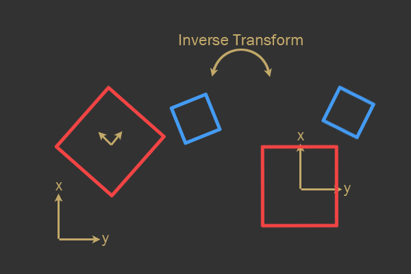
Inverse transformation from world space to model space of the red polygon. — Inverse transformation (left to right) from world space to model space of the red polygon.

As seen in the above image, if the inverse transformation of the red object is applied to both the red and blue polygons, then a collision detection test can be reduced to the form of an AABB vs OBB test, instead of computing complex math between two oriented shapes.

In much of the sample source code, vertices are constantly transformed from model to world and back to model, for all sorts of reasons. You should have a clear understanding of what this means in order to comprehend the sample collision detection code.

Collision Detection and Manifold Generation

In this section, I'll present quick outlines of polygon and circle collisions. Please see the sample source code for more in-depth implementation details.

Polygon to Polygon

Lets start with the most complex collision detection routine in this entire article series. The idea of checking for collision between two polygons is best done (in my opinion) with the Separating Axis Theorem (SAT).

However, instead of projecting each polygon's extents onto each other, there is a slightly newer and more efficient method, as outlined by Dirk Gregorius in his 2013 GDC Lecture (slides available here for free).

The first thing that must be learned is the concept of support points.

Support Points

The support point of a polygon is the vertex that is the farthest along a given direction. If two vertices have equal distances along the given direction, either one is acceptable.

In order to compute a supporting point, the dot product must be used to find a signed distance along a given direction. Since this is very simple, I'll show a quick example within this article:


// The extreme point along a direction within a polygon
Vec2 GetSupport( const Vec2& dir )
{
  real bestProjection = -FLT_MAX;
  Vec2 bestVertex;

  for(uint32 i = 0; i < m_vertexCount; ++i)
  {
    Vec2 v = m_vertices[i];
    real projection = Dot( v, dir );

    if(projection > bestProjection)
    {
      bestVertex = v;
      bestProjection = projection;
    }
  }

  return bestVertex;
}

The dot product is used on each vertex. The dot product represents a signed distance in a given direction, so the vertex with the greatest projected distance would be the vertex to return. This operation is performed in model space of the given polygon within the sample engine.

Finding Axis of Separation

By using the concept of support points, a search for the axis of separation can be performed between two polygons (polygon A and polygon B). The idea of this search is to loop along all faces of polygon A and find the support point in the negative normal to that face.

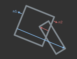
In the above image, two support points are shown: one on each object. The blue normal would correspond to the supporting point on the other polygon as the vertex farthest along in the opposite direction of the blue normal. Similarly, the red normal would be used to find the support point located at the end of the red arrow.

The distance from each supporting point to the current face would be the signed penetration. By storing the greatest distance a possible minimum axis of penetration can be recorded.

Here is an example function from the sample source code that finds the possible axis of minimum penetration using the GetSupport function:


real FindAxisLeastPenetration( uint32 *faceIndex, PolygonShape *A, PolygonShape *B )
{
  real bestDistance = -FLT_MAX;
  uint32 bestIndex;

  for(uint32 i = 0; i < A->m_vertexCount; ++i)
  {
    // Retrieve a face normal from A
    Vec2 n = A->m_normals[i];

    // Retrieve support point from B along -n
    Vec2 s = B->GetSupport( -n );

    // Retrieve vertex on face from A, transform into
    // B's model space
    Vec2 v = A->m_vertices[i];

    // Compute penetration distance (in B's model space)
    real d = Dot( n, s - v );

    // Store greatest distance
    if(d > bestDistance)
    {
      bestDistance = d;
      bestIndex = i;
    }
  }

  *faceIndex = bestIndex;
  return bestDistance;
}

Since this function returns the greatest penetration, if this penetration is positive that means the two shapes are not overlapping (negative penetration would signify no separating axis).

This function will need to be called twice, flipping A and B objects each call.

Clipping Incident and Reference Face

From here, the incident and reference face need to be identified, and the incident face needs to be clipped against the side planes of the reference face. This is a rather non-trivial operation, although Erin Catto (creator of Box2D, and all physics currently used by Blizzard) has created some great slides covering this topic in detail.

This clipping will generate two potential contact points. All contact points behind the reference face can be considered contact points.

Beyond Erin Catto's slides, the sample engine also has the clipping routines implemented as an example.

Circle to Polygon

The circle vs. polygon collision routine is quite a bit simpler than polygon vs. polygon collision detection. First, the closest face on the polygon to the center of the circle is computed in a similar way to using support points from the previous section: by looping over each face normal of the polygon and finding the distance from the circle's center to the face.

If the center of the circle is behind this closest face, specific contact information can be generated and the routine can immediately end.

After the closest face is identified, the test devolves into a line segment vs. circle test. A line segment has three interesting regions called Voronoi regions. Examine the following diagram:

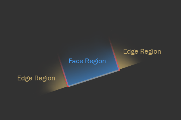
Intuitively, depending on where the center of the circle is located different contact information can be derived. Imagine the center of the circle is located on either vertex region. This means that the closest point to the circle's center will be an edge vertex, and the proper collision normal will be a vector from this vertex to the circle center.

If the circle is within the face region then the closest point of the segment to the circle's center will be the circle's center project onto the segment. The collision normal will just be the face normal.

To compute which Voronoi region the circle lies within, we use the dot product between a couple of vertices. The idea is to create an imaginary triangle and test to see whether the angle of the corner constructed with the segment's vertex is above or below 90 degrees. One triangle is created for each vertex of the line segment.

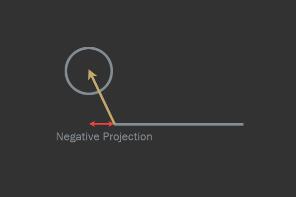
Projecting vector from edge vertex to circle center onto the edge.

A value of above 90 degrees will mean an edge region has been identified. If neither triangle's edge vertex angles is above 90 degrees, then the circle's center needs to be projected onto the segment itself to generate manifold information. As seen in the image above, if the vector from the edge vertex to the circle center dotted with the edge vector itself is negative, then the Voronoi region the circle lies within is known.

Luckily, the dot product can be used to compute a signed projection, and this sign will be negative if above 90 degrees and positive if below.

Collision Resolution

It is that time again: we'll return to our impulse resolution code for a third and final time. By now, you should be fully comfortable writing their own resolution code that computes resolution impulses, along with friction impulses, and can also can performed linear projection to resolve leftover penetration.

Rotational components need to be added to both the friction and penetration resolution. Some energy will be placed into angular velocity.

Here is our impulse resolution as we left it from the previous article on friction:

\[ Equation 5: \\
j = \frac{-(1 + e)((V^{A} - V^{B}) * t)}{\frac{1}{mass^{A}} + \frac{1}{mass^{B}}}
\]

If we throw in rotational components, the final equation looks like this:

\[ Equation 6: \\
j = \frac{-(1 + e)((V^{A} - V^{B}) * t)}{\frac{1}{mass^{A}} + \frac{1}{mass^{B}} + \frac{(r^{A} \times t)^{2}}{I^{A}} + \frac{(r^{B} \times t)^{2}}{I^{B}}}
\]

In the above equation, \(r\) is again a "radius", as in a vector from the COM of an object to the point of contact. A more in-depth derivation of this equation can be found on Chris Hecker's site.

It is important to realize that the velocity of a given point on an object is:

\[ Equation 7: \\
V' = V + \omega \times r
\]

The application of impulses changes slightly in order to account for the rotational terms:


void Body::ApplyImpulse( const Vec2& impulse, const Vec2& contactVector )
{
  velocity += 1.0f / mass * impulse;
  angularVelocity += 1.0f / inertia * Cross( contactVector, impulse );
}

Conclusion

This concludes the final article of this series. By now, quite a few topics have been covered, including impulse based resolution, manifold generation, friction, and orientation, all in two dimensions.

If you've made it this far, I must congratulate you! Physics engine programming for games is an extremely difficult area of study. I wish all readers luck, and again please feel free to comment or ask questions below.