Today’s post is by Thomas Yokota, an epidemiologist in Hawaii. I’ve been corresponding with Thomas via email and telephone for a while. I asked Thomas if he could write an introduction to how R, mapping and open data are used in the public health community. This is his reply.
[content_upgrade cu_id=”2764″]Bonus: Download the code from this post![content_upgrade_button]Click Here[/content_upgrade_button][/content_upgrade]
What is public health?
Public health is a broad and sometimes overreaching field. Consequently, I am asked, “what is public health?” more so than “what school did you go to (in Hawaii)?” With that said, I’d like to start off with a quote by C.E. Taylor:
“The focus of public health is the community. The ‘patient’ is a whole population unit. The shift in professional orientation which occurs as the unit of attention moves from the individual to the group must be clearly recognized and explicitly stated because it has led to many misunderstandings in the past.”
Once it’s clearly understood that public health is not brain surgery and – according to the CDC – more about zombie invasions, the next response I usually get is, “so what does public health do if it doesn’t cure diabetes?” Such a loaded question. In a nutshell, the four core functions of public health are as follows:
- Assessment
- Policy development
- Assurance
- Communication
In other words, public health professionals rely on studies and surveys, such as the Behavioral Risk Factors Surveillance System (BRFSS), to understand health trends. Consequently, campaigns and/or policies are developed to break trends when needed.
So why R?
R is a great asset for making powerful graphs and maps, and can complement current SAS/STATA/SPSS/etc. workflows. Proprietary statistical programs will always be public health’s frenemies in the area of research and complex survey analysis – it’s inevitable that we must sacrifice funding health fair incentives to pay for license fees – but let’s not write off R too soon. R is also desirable for pubic health data analysts (i.e., epidemiologists) who work in community organizations.
BRFSS
In laymen terms, many public health organizations and professionals cite the BRFSS when interested in health risk behaviors, health access and chronic disease prevalence. Introductions and examples have already been created on BRFSS for R, and have been featured on R-bloggers. Anthony Damico maintains a GitHub repository on downloading and storing complex surveys. I recommend his solution for those who are new to R and/or complex survey analysis and because there is a significant speed increase when working on analyzing the BRFSS alongside MonetDB. I also recommend Dr. Thomas Lumley’s book Complex Survey Analysis to understand complex surveys.
load dependencies and data
In this example, I am taking a couple of shortcuts to import the data and to test out the srvyr package because… pipes. It also helps me to cut down some of the code and instructions entailed to setting up R and MonetDB – it’s also been done before. It is important to note, however, that Survey package is doing all the heavy lifting.
I use pacman package when handling all additional package loading and installs. I find it to be more convenient than library(). I am also borrowing Anthony’s download script to pull the BRFSS from CDC before loading it into R.
install.packages('pacman')
pacman::p_load(RCurl, foreign, downloader, survey, srvyr, ggplot2, dplyr)
source_url("https://raw.githubusercontent.com/ajdamico/asdfree/master/Download%20Cache/download%20cache.R", prompt=F, echo=F)
# download ez-pz brought to you by anthony joseph damico [[email protected]]
tf <- tempfile()
td <- tempdir()
xpt <- "http://www.cdc.gov/brfss/annual_data/2014/files/LLCP2014XPT.ZIP"
download_cached(xpt, tf, mode='wb')
local.fn <- unzip(tf, exdir=td)
brfss14 <- read.xport(local.fn)
state.id <- read.csv("https://raw.githubusercontent.com/tyokota/complexsurvey/master/brfss_state.csv", stringsAsFactors=F)
ageg65yr.id <- read.csv("https://raw.githubusercontent.com/tyokota/complexsurvey/master/ageg65yr.csv", stringsAsFactors=F)
create the survey object
The usual practice is to use SAS-callable SUDAAN to handle the sampling design and weighting; however, we can also do this in R. In this example, I will look at BMI categories as inferred by the following variable and question: BMI5CAT-Computed body mass index categories, which has been re-coded to compare overweight and/or obese prevalence.
brfss.design14 <- brfss14 %>%
  as_survey_design(ids=X_PSU,
                   weight=X_LLCPWT,
                   nest=T,
                   strata=X_STSTR,
                   variables= c(X_BMI5CAT, X_MRACE1, X_STATE, X_AGEG5YR))
brfss.design14 <- brfss.design14 %>%
  mutate(X_BMI5CAT2  = car::recode(X_BMI5CAT, "c(3,4)=1; NA=NA;  else=0"),
         X_BMI5CAT2  = as.factor(X_BMI5CAT2),
         X_BMI5CAT2a = car::recode(X_BMI5CAT2, "1='Obese/overweight'; NA=NA; else='Not Obese/overweight'"),
         X_BMI5CAT2a = factor(X_BMI5CAT2a, levels=c('Obese/overweight', 'Not Obese/overweight'), ordered=TRUE),
         X_MRACE1a   = car::recode(X_MRACE1, "1='White'; 2='Black'; 3='AIAN'; 4='Asian'; 5='NHOPI';  NA=NA; c(6,7)='other/multiracial'; else=NA"),
         X_AGEG5YR   = car::recode(X_AGEG5YR, "1='Age 18 to 24'; 2='Age 25 to 29'; 3='Age 30 to 34'; 4='Age 35 to 39'; 5='Age 40 to 44'; 6='Age 45 to 49'; 7='Age 50 to 54'; 8='Age 55 to 59'; 9='Age 60 to 64'; 10='Age 65 to 69'; 11='Age 70 to 74'; 12='Age 75 to 79'; 13='Age 80 or older'; 14='Dont know/Refused/Missing'"))
state-by-state comparison
Now that we have created the survey design object, we can use R to create estimates from the data.
options(survey.lonely.psu = "certainty")
state.bmi <- brfss.design14 %>%
group_by(X_STATE, X_BMI5CAT2) %>%
summarize(prevalence = survey_mean(na.rm=T, vartype = c("ci")),
N = survey_total(na.rm=T)) %>%
mutate(X_STATE = as.character(X_STATE))
data(county.regions, package="choroplethrMaps")
county.regions <- county.regions %>%
select(state.fips.character, state.name) %>% unique
state.bmi <- state.bmi %>%
mutate(X_STATE = str_pad(X_STATE, 2, side="left", pad="0")) %>%
left_join(county.regions, by=c("X_STATE"="state.fips.character")) %>%
mutate(state.name = ifelse(X_STATE=="72", "puerto rico",
ifelse(X_STATE=="66", "guam", state.name)))
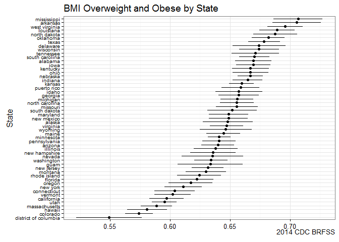
ggplot(subset(state.bmi, X_BMI5CAT2==1), aes(y=reorder(state.name, prevalence), x=prevalence, xmin=prevalence_low, xmax=prevalence_upp)) +
geom_point() +
geom_errorbarh(height=0) +
labs(y="State", x=NULL,
title="BMI Overweight and Obese by State",
caption="2014 CDC BRFSS") +
theme_bw() +
theme(axis.text.y=element_text(size=rel(0.8)))
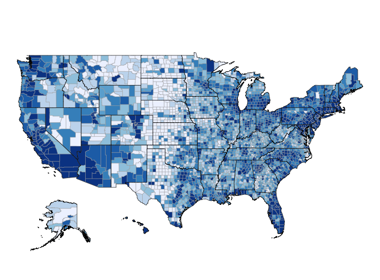
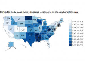
BRFSS is commonly used to make state-by-state comparisons, such as state-by-state rankings. Most recently, choropleth maps have been used to visualize prevalence rates across the nation.
state.bmi2 <- state.bmi %>%
  filter(X_BMI5CAT2==1) %>%
  select(region=state.name, value=prevalence)
choroplethr::state_choropleth(state.bmi2, title="Computed body mass index categories (overweight or obese) choropleth map", num_colors=9)
deep dive Hawaii – stratify by race
Before we start dropping leaflets on healthy eating across the Bible Belt, why don’t we dig into the data a bit more. Let’s take my home state for example. When comparing states, Hawaii ranks low in obesity and overweight prevalence.
As a reminder: you can always verify your query against the [CDC BRFSS Prevalence & Trends Tool](http://www.cdc.gov/brfss/brfssprevalence/index.html).
hawaii.bmi <- brfss.design14 %>%
  filter(X_STATE==15, X_MRACE1a %in% c("NHOPI", "White", "Asian", "Dont know/Refused/Missing")) %>%
  group_by(X_MRACE1a, X_BMI5CAT2a) %>%
  summarize(prevalence = survey_mean(na.rm=T),
            N = survey_total(na.rm=T),
            prevalence_ci = survey_mean(na.rm=T, vartype = c("ci")))
ggplot(subset(hawaii.bmi, X_BMI5CAT2a=="Obese/overweight"), aes(y=X_MRACE1a, x=prevalence, xmin=prevalence_ci_low, xmax=prevalence_ci_upp, colour=X_MRACE1a)) +
geom_point() +
geom_errorbarh(height=0) +
labs(y="Race", x=NULL,
     title="BMI Overweight and Obese in State of Hawaii by Race",
     caption="2014 CDC BRFSS") +
theme_bw() +
theme(axis.text.y=element_text(size=rel(0.8)))
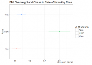
Stratifying by race shows us a different picture: Native Hawaiians and Other Pacific Islanders (NHOPI) overweight/obese prevalence is at 80% (CI95%: 73-87%), easily topping all point estimates by state.
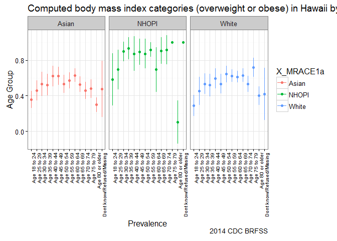
deep dive Hawaii – stratify by race and age group
Going one level deeper, we see that onset of Going one level deeper, we see that onset of overweight/obesity starts earlier for NHOPI and that prevalence across age groups is higher in comparison to other groups. The graph suggests that efforts to address overweight/obesity among NHOPI groups is needed in Hawaii; in addition, it also suggests that NHOPIs would benefit from intervention at earlier stages in life.
hawaii.bmi2 <- brfss.design14 %>%
  filter(X_STATE==15, X_MRACE1a %in% c("NHOPI", "White", "Asian", "Dont know/Refused/Missing")) %>%
  group_by(X_MRACE1a, X_AGEG5YR, X_BMI5CAT2a) %>%
  summarize(prevalence = survey_mean(na.rm=T),
            N = survey_total(na.rm=T),
            prevalence_ci = survey_mean(na.rm=T, vartype = c("ci")))
ggplot(subset(hawaii.bmi2, X_BMI5CAT2a=="Obese/overweight"), aes(y=X_AGEG5YR, x=prevalence, xmin=prevalence_ci_low, xmax=prevalence_ci_upp, colour=X_MRACE1a)) +
geom_point() +
geom_errorbarh(height=0) +
coord_flip() +
labs(y="Race", x=NULL,
     title="BMI Overweight and Obese in State of Hawaii by Race",
     caption="2014 CDC BRFSS") +
  facet_grid(~X_MRACE1a) +
theme_bw() +
ylab("Prevalence") +
xlab("Age Group") +
ggtitle("Computed body mass index categories (overweight or obese) in Hawaii by race and age") +
theme(axis.text.x = element_text(angle = 90, hjust = 1),
      panel.background = element_rect(fill = 'white' )) +
guides(fill = guide_legend(title = "Categories")) +
theme(axis.text.x=element_text(size=rel(0.8)))

Conclusion
Relying on high-level estimates alone can sometimes mislead your agenda. For example, after stratifying by race, we saw that the shared benefits of living in Hawaii were not equally shared by all groups. Further stratifying by age shows that onset by race occurred earlier for NHOPIs. These cuts of the data can help to narrow down public health efforts and hopefully prevent the usual spray-and-pray approach to solving problems.
[content_upgrade cu_id=”2764″]Bonus: Download the code from this post![content_upgrade_button]Click Here[/content_upgrade_button][/content_upgrade]