


There are many reasons you might want to create a custom physics engine: first, learning and honing your skills in mathematics, physics and programming are great reasons to attempt such a project; second, a custom physics engine can tackle any sort of technical effect the creator has the skill to create. In this article I would like to provide a solid introduction on how to create a custom physics engine entirely from scratch.
Physics provides a wonderful means for allowing a player to immerse themselves within a game. It makes sense that a mastery of a physics engine would be a powerful asset for any programmer to have at their disposal. Optimizations and specializations can be made at any time due to a deep understanding of the inner workings of the physics engine.
By the end of this tutorial the following topics will have been covered, in two dimensions:
- Simple collision detection
- Simple manifold generation
- Impulse resolution
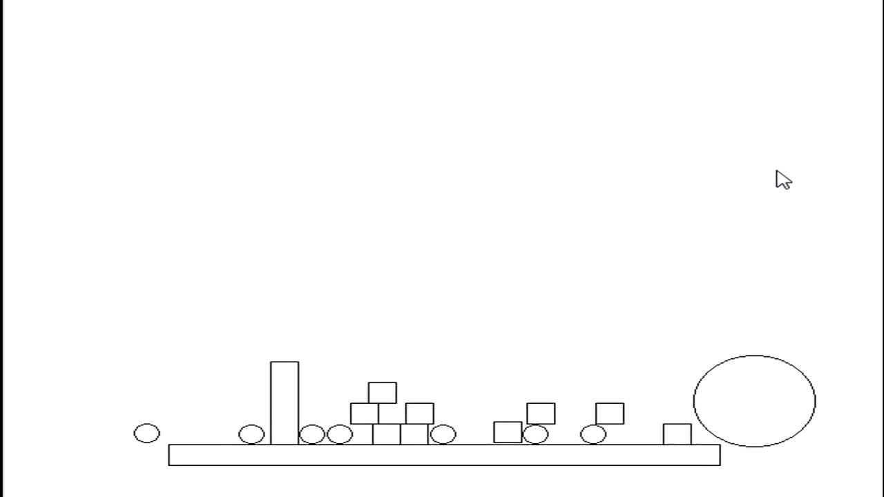
Here's a quick demo:
Note: Although this tutorial is written using C++, you should be able to use the same techniques and concepts in almost any game development environment.
Prerequisites
This article involves a fair amount of mathematics and geometry, and to a much lesser extent actual coding. A couple prerequisites for this article are:
- A basic understanding of simple vector math
- The ability to perform algebraic math
Collision Detection
There are quite a few articles and tutorials throughout the internet, including here on Tuts+, that cover collision detection. Knowing this, I would like to run through the topic very quickly as this section is not the focus of this article.
Axis Aligned Bounding Boxes
An Axis Aligned Bounding Box (AABB) is a box that has its four axes aligned with the coordinate system in which it resides. This means it is a box that cannot rotate, and is always squared off at 90 degrees (usually aligned with the screen). In general it is referred to as a "bounding box" because AABBs are used to bound other more complex shapes.
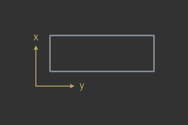

The AABB of a complex shape can be used as a simple test to see if more complex shapes inside the AABBs can possibly be intersecting. However in the case of most games the AABB is used as a fundamental shape, and does not actually bound anything else. The structure of your AABB is important. There are a few different ways to represent an AABB, however this is my favorite:
1 |
struct AABB |
2 |
{
|
3 |
Vec2 min; |
4 |
Vec2 max; |
5 |
};
|
This form allows an AABB to be represented by two points. The min point represents the lower bounds of the x and y axis, and max represents the higher bounds - in other words, they represent the top left and bottom right corners. In order to tell whether two AABB shapes are intersecting you will need to have a basic understanding of the Separating Axis Theorem (SAT).
Here's a quick test taken from Real-Time Collision Detection by Christer Ericson, which makes use of the SAT:
1 |
bool AABBvsAABB( AABB a, AABB b ) |
2 |
{
|
3 |
// Exit with no intersection if found separated along an axis
|
4 |
if(a.max.x < b.min.x or a.min.x > b.max.x) return false |
5 |
if(a.max.y < b.min.y or a.min.y > b.max.y) return false |
6 |
|
7 |
// No separating axis found, therefor there is at least one overlapping axis
|
8 |
return true |
9 |
}
|
Circles
A circle is represented by a radius and point. Here is what your circle structure ought to look like:
1 |
struct Circle |
2 |
{
|
3 |
float radius |
4 |
Vec position |
5 |
};
|
Testing for whether or not two circles intersect is very simple: take the radii of the two circles and add them together, then check to see if this sum is greater than the distance between the two circles.
An important optimization to make here is get rid of any need to use the square root operator:
1 |
float Distance( Vec2 a, Vec2 b ) |
2 |
{
|
3 |
return sqrt( (a.x - b.x)^2 + (a.y - b.y)^2 ) |
4 |
}
|
5 |
|
6 |
bool CirclevsCircleUnoptimized( Circle a, Circle b ) |
7 |
{
|
8 |
float r = a.radius + b.radius |
9 |
return r < Distance( a.position, b.position ) |
10 |
}
|
11 |
|
12 |
bool CirclevsCircleOptimized( Circle a, Circle b ) |
13 |
{
|
14 |
float r = a.radius + b.radius |
15 |
r *= r |
16 |
return r < (a.x + b.x)^2 + (a.y + b.y)^2 |
17 |
}
|
In general multiplication is a much cheaper operation than taking the square root of a value.
Impulse Resolution
Impulse resolution is a particular type of collision resolution strategy. Collision resolution is the act of taking two objects who are found to be intersecting and modifying them in such a way as to not allow them to remain intersecting.
In general an object within a physics engine has three main degrees of freedom (in two dimensions): movement in the xy plane and rotation. In this article we implicitly restrict rotation and use just AABBs and Circles, so the only degree of freedom we really need to consider is movement along the xy plane.
By resolving detected collisions we place a restriction upon movement such that objects cannot remain intersecting one another. The idea behind impulse resolution is to use an impulse (instantaneous change in velocity) to separate objects found colliding. In order to do this the mass, position, and velocity of each object must be taken into account somehow: we want large objects colliding with smaller ones to move a little bit during collision, and to send the small objects flying away. We also want objects with infinite mass to not move at all.

In order to achieve such effects and follow along with natural intuition of how objects behave we'll use rigid bodies and a fair bit of math. A rigid body is just a shape defined by the user (that is, by you, the developer) that is implicitly defined to be non-deformable. Both AABBs and Circles in this article are non-deformable, and will always be either an AABB or Circle. No squashing or stretching allowed.
Working with rigid bodies allows for a lot of math and derivations to be heavily simplified. This is why rigid bodies are commonly used in game simulations, and why we'll be using them in this article.
Our Objects Collided - Now What?
Assuming we have two shapes found to be intersecting, how does one actually separate the two? Lets assume our collision detection provided us with two important pieces of information:
- Collision normal
- Penetration depth
In order to apply an impulse to both objects and move them apart, we need to know what direction to push them and by how much. The collision normal is the direction in which the impulse will be applied. The penetration depth (along with some other things) determine how large of an impulse will be used. This means the only value that needs to be solved for is the magnitude of our impulse.
Now let's go on a long trek to discover how we can solve for this impulse magnitude. We'll start with our two objects that have been found to be intersecting:
\[ V^{AB} = V^B - V^A \] Note that in order to create a vector from position A to position B, you must do: endpoint - startpoint. \(V^{AB}\) is the relative velocity from A to B. This equation ought to be expressed in terms of the collision normal \(n\) - that is, we would like to know the relative velocity from A to B along the collision normal's direction:
\[ V^{AB} \cdot n = (V^B - V^A) \cdot n \]
We are now making use of the dot product. The dot product is simple; it is the sum of component-wise products:
\[ V_1 = \begin{bmatrix}x_1 \\y_1\end{bmatrix}, V_2 = \begin{bmatrix}x_2 \\y_2\end{bmatrix} \\ V_1 \cdot V_2 = x_1 * x_2 + y_2 * y_2 \]
The next step is to introduce what is called the coefficient of restitution. Restitution is a term that means elasticity, or bounciness. Each object in your physics engine will have a restitution represented as a decimal value. However only one decimal value will be used during the impulse calculation.
To decide what restitution to use (denoted by \(e\) for epsilon), you should always use the lowest restitution involved in the collision for intuitive results:
1 |
// Given two objects A and B
|
2 |
e = min( A.restitution, B.restitution ) |
Once \(e\) is acquired we can place it into our equation solving for the impulse magnitude.
Newton's Law of Restitution states the following:
\[V' = e * V \]
All this is saying is that the velocity after a collision is equal to the velocity before it, multiplied by some constant. This constant represents a "bounce factor". Knowing this, it becomes fairly simple to integrate restitution into our current derivation:
\[ V^{AB} \cdot n = -e * (V^B - V^A) \cdot n \]
Notice how we introduced a negative sign here. In Newton's Law of Restitution, \(V'\), the resulting vector after the bounce, is actually going in the opposite direction of V. So how do we represent opposite directions in our derivation? Introduce a negative sign.
So far so good. Now we need to be able to express these velocities while under the influence of an impulse. Here's a simple equation for modify a vector by some impulse scalar \(j\) along a specific direction \(n\):
\[ V' = V + j * n \]
Hopefully the above equation makes sense, as it is very important to understand. We have a unit vector \(n\) which represents a direction. We have a scalar \(j\) which represents how long our \(n\) vector will be. We then add our scaled \(n\) vector to \(V\) to result in \(V'\). This is just adding one vector onto another, and we can use this small equation to apply an impulse of one vector to another.
There's a little more work to be done here. Formally, an impulse is defined as a change in momentum. Momentum is mass * velocity. Knowing this, we can represent an impulse as it is formally defined like so:
\[ Impulse = mass * Velocity \\ Velocity = \frac{Impulse}{mass} \therefore V' = V + \frac{j * n}{mass}\]
Good progress has been made so far! However we need to be able to express an impulse using \(j\) in terms of two different objects. During a collision with object A and B, A will be pushed in the opposite direction of B:
\[ V'^A = V^A + \frac{j * n}{mass^A} \\ V'^B = V^B - \frac{j * n}{mass^B} \]
These two equations will push A away from B along the direction unit vector \(n\) by impulse scalar (magnitude of \(n\)) \(j\).
All that is now required is to merge Equations 8 and 5. Our resulting equation will look something like this:
\[ (V^A - V^V + \frac{j * n}{mass^A} + \frac{j * n}{mass^B}) * n = -e * (V^B - V^A) \cdot n \\ \therefore \\ (V^A - V^V + \frac{j * n}{mass^A} + \frac{j * n}{mass^B}) * n + e * (V^B - V^A) \cdot n = 0 \]
If you recall, the original goal was to isolate our magnitude. This is because we know what direction to resolve the collision in (assumed given by the collision detection), and only have left to solve the magnitude of this direction. The magnitude which is an unknown in our case is \(j\); we must isolate \(j\) and solve for it.
\[ (V^B - V^A) \cdot n + j * (\frac{j * n}{mass^A} + \frac{j * n}{mass^B}) * n + e * (V^B - V^A) \cdot n = 0 \\ \therefore \\ (1 + e)((V^B - V^A) \cdot n) + j * (\frac{j * n}{mass^A} + \frac{j * n}{mass^B}) * n = 0 \\ \therefore \\ j = \frac{-(1 + e)((V^B - V^A) \cdot n)}{\frac{1}{mass^A} + \frac{1}{mass^B}} \]
Whew! That was a fair bit of math! It is all over for now though. It's important to notice that in the final version of Equation 10 we have \(j\) on the left (our magnitude) and everything on the right is all known. This means we can write a few lines of code to solve for our impulse scalar \(j\). And boy is the code a lot more readable than mathematical notation!
1 |
void ResolveCollision( Object A, Object B ) |
2 |
{
|
3 |
// Calculate relative velocity
|
4 |
Vec2 rv = B.velocity - A.velocity |
5 |
|
6 |
// Calculate relative velocity in terms of the normal direction
|
7 |
float velAlongNormal = DotProduct( rv, normal ) |
8 |
|
9 |
// Do not resolve if velocities are separating
|
10 |
if(velAlongNormal > 0) |
11 |
return; |
12 |
|
13 |
// Calculate restitution
|
14 |
float e = min( A.restitution, B.restitution) |
15 |
|
16 |
// Calculate impulse scalar
|
17 |
float j = -(1 + e) * velAlongNormal |
18 |
j /= 1 / A.mass + 1 / B.mass |
19 |
|
20 |
// Apply impulse
|
21 |
Vec2 impulse = j * normal |
22 |
A.velocity -= 1 / A.mass * impulse |
23 |
B.velocity += 1 / B.mass * impulse |
24 |
}
|
There are a few key things to note in the above code sample. The first thing is the check on Line 10, if(VelAlongNormal > 0). This check is very important; it makes sure that you only resolve a collision if the objects are moving towards each other.

If objects are moving away from one another we want to do nothing. This will prevent objects that shouldn't actually be considered colliding from resolving away from one another. This is important for creating a simulation that follows human intuition on what should happen during object interaction.
The second thing to note is that inverse mass is computed multiple times for no reason. It is best to just store your inverse mass within each object and pre-compute it one time:
1 |
A.inv_mass = 1 / A.mass |
1/mass. The last thing to note is that we intelligently distribute our impulse scalar \(j\) over the two objects. We want small objects to bounce off of big objects with a large portion of \(j\), and the big objects to have their velocities modified by a very small portion of \(j\).
In order to do this you could do:
1 |
float mass_sum = A.mass + B.mass |
2 |
float ratio = A.mass / mass_sum |
3 |
A.velocity -= ratio * impulse |
4 |
|
5 |
ratio = B.mass / mass_sum |
6 |
B.velocity += ratio * impulse |
It is important to realize that the above code is equivalent to the ResolveCollision() sample function from before. Like stated before, inverse masses are quite useful in a physics engine.
Sinking Objects
If we go ahead and use the code we have so far, objects will run into each other and bounce off. This is great, although what happens if one of the objects has infinite mass? Well we need a good way to represent infinite mass within our simulation.
I suggest using zero as infinite mass - although if we try to compute inverse mass of an object with zero we will have a division by zero. The workaround to this is to do the following when computing inverse mass:
1 |
if(A.mass == 0) |
2 |
A.inv_mass = 0 |
3 |
else
|
4 |
A.inv_mass = 1 / A.mass |
A value of zero will result in proper calculations during impulse resolution. This is still okay. The problem of sinking objects arises when something starts sinking into another object due to gravity. Perhaps something with low restitution hits a wall with infinite mass and begins to sink.
This sinking is due to floating point errors. During each floating point calculation a small floating point error is introduced due to hardware. (For more information, Google [Floating point error IEEE754].) Over time this error accumulates in positional error, causing objects to sink into one another.
In order to correct this error it must be accounted for. To correct this positional error I will show you a method called linear projection. Linear projection reduces the penetration of two objects by a small percentage, and this is performed after the impulse is applied. Positional correction is very simple: move each object along the collision normal \(n\) by a percentage of the penetration depth:
1 |
void PositionalCorrection( Object A, Object B ) |
2 |
{
|
3 |
const float percent = 0.2 // usually 20% to 80% |
4 |
Vec2 correction = penetrationDepth / (A.inv_mass + B.inv_mass)) * percent * n |
5 |
A.position -= A.inv_mass * correction |
6 |
B.position += B.inv_mass * correction |
7 |
}
|
Note that we scale the penetrationDepth by the total mass of the system. This will give a positional correction proportional to how much mass we are dealing with. Small objects push away faster than heavier objects.
There is a slight problem with this implementation: if we are always resolving our positional error then objects will jitter back and forth while they rest upon one another. In order to prevent this some slack must be given. We only perform positional correction if the penetration is above some arbitrary threshold, referred to as "slop":
1 |
void PositionalCorrection( Object A, Object B ) |
2 |
{
|
3 |
const float percent = 0.2 // usually 20% to 80% |
4 |
const float slop = 0.01 // usually 0.01 to 0.1 |
5 |
Vec2 correction = max( penetration - k_slop, 0.0f ) / (A.inv_mass + B.inv_mass)) * percent * n |
6 |
A.position -= A.inv_mass * correction |
7 |
B.position += B.inv_mass * correction |
8 |
}
|
This allows objects to penetrate ever so slightly without the position correction kicking in.
Simple Manifold Generation
The last topic to cover in this article is simple manifold generation. A manifold in mathematical terms is something along the lines of "a collection of points that represents an area in space". However, when I refer to the term manifold I am referring to a small object that contains information about a collision between two objects.
Here is a typical manifold setup:
1 |
struct Manifold |
2 |
{
|
3 |
Object *A; |
4 |
Object *B; |
5 |
float penetration; |
6 |
Vec2 normal; |
7 |
};
|
During collision detection, both penetration and the collision normal should be computed. In order to find this info the original collision detection algorithms from the top of this article must be extended.
Circle vs Circle
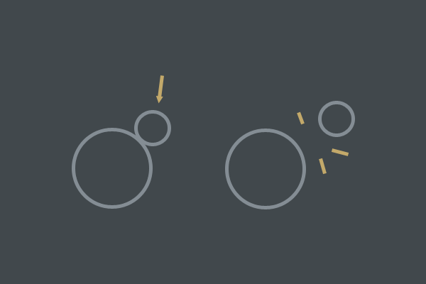
Lets start with the simplest collision algorithm: Circle vs Circle. This test is mostly trivial. Can you imagine what the direction to resolve the collision will be in? It is the vector from Circle A to Circle B. This can be obtained by subtracting B's position from A's.
Penetration depth is related to the Circles' radii and distance from one another. The overlap of the Circles can be computed by subtracting the summed radii by the distance from each object.
Here is a full sample algorithm for generating the manifold of a Circle vs Circle collision:
1 |
bool CirclevsCircle( Manifold *m ) |
2 |
{
|
3 |
// Setup a couple pointers to each object
|
4 |
Object *A = m->A; |
5 |
Object *B = m->B; |
6 |
|
7 |
// Vector from A to B
|
8 |
Vec2 n = B->pos - A->pos |
9 |
|
10 |
float r = A->radius + B->radius |
11 |
r *= r |
12 |
|
13 |
if(n.LengthSquared( ) > r) |
14 |
return false |
15 |
|
16 |
// Circles have collided, now compute manifold
|
17 |
float d = n.Length( ) // perform actual sqrt |
18 |
|
19 |
// If distance between circles is not zero
|
20 |
if(d != 0) |
21 |
{
|
22 |
// Distance is difference between radius and distance
|
23 |
m->penetration = r - d |
24 |
|
25 |
// Utilize our d since we performed sqrt on it already within Length( )
|
26 |
// Points from A to B, and is a unit vector
|
27 |
c->normal = t / d |
28 |
return true |
29 |
}
|
30 |
|
31 |
// Circles are on same position
|
32 |
else
|
33 |
{
|
34 |
// Choose random (but consistent) values
|
35 |
c->penetration = A->radius |
36 |
c->normal = Vec( 1, 0 ) |
37 |
return true |
38 |
}
|
39 |
}
|
The most notable things here are: we do not perform any square roots until necessary (objects are found to be colliding), and we check to make sure the circles are not on the same exact position. If they are on the same position our distance would be zero, and we must avoid division by zero when we compute t / d.
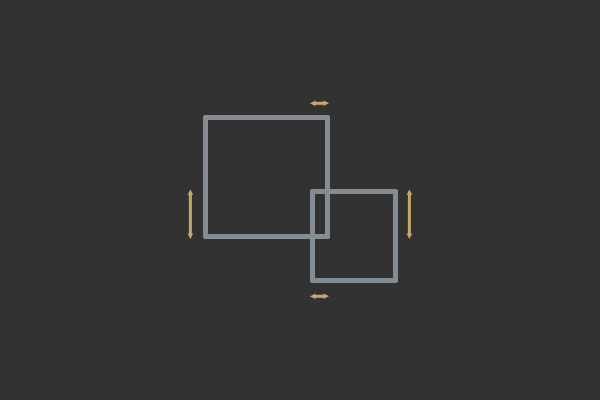
AABB vs AABB
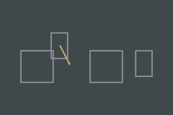
The AABB to AABB test is a little more complex than Circle vs Circle. The collision normal will not be the vector from A to B, but will be a face normal. An AABB is a box with four faces. Each face has a normal. This normal represents a unit vector that is perpendicular to the face.
Examine the general equation of a line in 2D:
\[ ax + by + c = 0 \\ normal = \begin{bmatrix}a \\b\end{bmatrix} \]
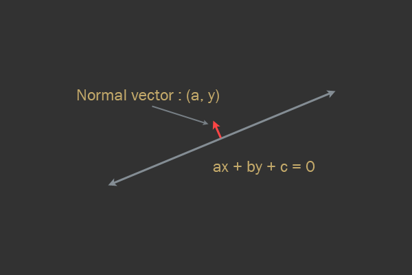

In the above equation, a and b are the normal vector for a line, and the vector (a, b) is assumed to be normalized (length of vector is zero). Again, our collision normal (direction to resolve the collision) will be in the direction of one of the face normals.
c represents in the general equation of a line? c is the distance from the origin. This is very useful for testing to see if a point is on one side of a line or another, as you will see in the next article.Now all that is needed is to find out which face is colliding on one of the objects with the other object, and we have our normal. However sometimes multiple faces of two AABBs can intersect, such as when two corners intersect each other. This means we must find the axis of least penetration.

Here is a full algorithm for AABB to AABB manifold generation and collision detection:


1 |
bool AABBvsAABB( Manifold *m ) |
2 |
{
|
3 |
// Setup a couple pointers to each object
|
4 |
Object *A = m->A |
5 |
Object *B = m->B |
6 |
|
7 |
// Vector from A to B
|
8 |
Vec2 n = B->pos - A->pos |
9 |
|
10 |
AABB abox = A->aabb |
11 |
AABB bbox = B->aabb |
12 |
|
13 |
// Calculate half extents along x axis for each object
|
14 |
float a_extent = (abox.max.x - abox.min.x) / 2 |
15 |
float b_extent = (bbox.max.x - bbox.min.x) / 2 |
16 |
|
17 |
// Calculate overlap on x axis
|
18 |
float x_overlap = a_extent + b_extent - abs( n.x ) |
19 |
|
20 |
// SAT test on x axis
|
21 |
if(x_overlap > 0) |
22 |
{
|
23 |
// Calculate half extents along x axis for each object
|
24 |
float a_extent = (abox.max.y - abox.min.y) / 2 |
25 |
float b_extent = (bbox.max.y - bbox.min.y) / 2 |
26 |
|
27 |
// Calculate overlap on y axis
|
28 |
float y_overlap = a_extent + b_extent - abs( n.y ) |
29 |
|
30 |
// SAT test on y axis
|
31 |
if(y_overlap > 0) |
32 |
{
|
33 |
// Find out which axis is axis of least penetration
|
34 |
if(x_overlap > y_overlap) |
35 |
{
|
36 |
// Point towards B knowing that n points from A to B
|
37 |
if(n.x < 0) |
38 |
m->normal = Vec2( -1, 0 ) |
39 |
else
|
40 |
m->normal = Vec2( 0, 0 ) |
41 |
m->penetration = x_overlap |
42 |
return true |
43 |
}
|
44 |
else
|
45 |
{
|
46 |
// Point toward B knowing that n points from A to B
|
47 |
if(n.y < 0) |
48 |
m->normal = Vec2( 0, -1 ) |
49 |
else
|
50 |
m->normal = Vec2( 0, 1 ) |
51 |
m->penetration = y_overlap |
52 |
return true |
53 |
}
|
54 |
}
|
55 |
}
|
56 |
}
|
Circle vs AABB
The last test I will cover is the Circle vs AABB test. The idea here is to compute the closest point on the AABB to the Circle; from there the test devolves into something similar to the Circle vs Circle test. Once the closest point is computed and a collision is detected the normal is the direction of the closest point to the circle's center. The penetration depth is the difference between the distance of the closest point to the circle and the radius of the circle.


There is one tricky special case; if the circle's center is within the AABB then the center of the circle needs to be clipped to the closest edge of the AABB, and the normal needs to be flipped.
1 |
bool AABBvsCircle( Manifold *m ) |
2 |
{
|
3 |
// Setup a couple pointers to each object
|
4 |
Object *A = m->A |
5 |
Object *B = m->B |
6 |
|
7 |
// Vector from A to B
|
8 |
Vec2 n = B->pos - A->pos |
9 |
|
10 |
// Closest point on A to center of B
|
11 |
Vec2 closest = n |
12 |
|
13 |
// Calculate half extents along each axis
|
14 |
float x_extent = (A->aabb.max.x - A->aabb.min.x) / 2 |
15 |
float y_extent = (A->aabb.max.y - A->aabb.min.y) / 2 |
16 |
|
17 |
// Clamp point to edges of the AABB
|
18 |
closest.x = Clamp( -x_extent, x_extent, closest.x ) |
19 |
closest.y = Clamp( -y_extent, y_extent, closest.y ) |
20 |
|
21 |
bool inside = false |
22 |
|
23 |
// Circle is inside the AABB, so we need to clamp the circle's center
|
24 |
// to the closest edge
|
25 |
if(n == closest) |
26 |
{
|
27 |
inside = true |
28 |
|
29 |
// Find closest axis
|
30 |
if(abs( n.x ) > abs( n.y )) |
31 |
{
|
32 |
// Clamp to closest extent
|
33 |
if(closest.x > 0) |
34 |
closest.x = x_extent |
35 |
else
|
36 |
closest.x = -x_extent |
37 |
}
|
38 |
|
39 |
// y axis is shorter
|
40 |
else
|
41 |
{
|
42 |
// Clamp to closest extent
|
43 |
if(closest.y > 0) |
44 |
closest.y = y_extent |
45 |
else
|
46 |
closest.y = -y_extent |
47 |
}
|
48 |
}
|
49 |
|
50 |
Vec2 normal = n - closest |
51 |
real d = normal.LengthSquared( ) |
52 |
real r = B->radius |
53 |
|
54 |
// Early out of the radius is shorter than distance to closest point and
|
55 |
// Circle not inside the AABB
|
56 |
if(d > r * r && !inside) |
57 |
return false |
58 |
|
59 |
// Avoided sqrt until we needed
|
60 |
d = sqrt( d ) |
61 |
|
62 |
// Collision normal needs to be flipped to point outside if circle was
|
63 |
// inside the AABB
|
64 |
if(inside) |
65 |
{
|
66 |
m->normal = -n |
67 |
m->penetration = r - d |
68 |
}
|
69 |
else
|
70 |
{
|
71 |
m->normal = n |
72 |
m->penetration = r - d |
73 |
}
|
74 |
|
75 |
return true |
76 |
}
|
Conclusion
Hopefully by now you've learned a thing or two about physics simulation. This tutorial is enough to let you set up a simple custom physics engine made entirely from scratch. In the next part, we will be covering all the necessary extensions that all physics engines require, including:
- Contact pair sorting and culling
- Broadphase
- Layering
- Integration
- Timestepping
- Halfspace intersection
- Modular design (materials, mass and forces)
I hope you enjoyed this article and I look forward to answering questions in the comments.


