How to Create a Custom 2D Physics Engine: The Core Engine

In this part of my series on creating a custom 2D physics engine for your games, we'll add more features to the impulse resolution we got working in the first part. In particular, we'll look at integration, timestepping, using a modular design for our code, and broad phase collision detection.

Introduction

In the last post in this series I covered the topic of impulse resolution. Read that first, if you haven't already!

Let's dive straight into the topics covered in this article. These topics are all of the necessities of any half-decent physics engine, so now is an appropriate time to build more features on top of the core resolution from the last article.

Integration
Timestepping
Modular Design
- Bodies
- Shapes
- Forces
- Materials
Broad Phase
- Contact pair duplicate culling
- Layering
Halfspace Intersection Test

Integration

Integration is entirely simple to implement, and there are very many areas on the internet that provide good information for iterative integration. This section will mostly show how to implement a proper integration function, and point to some different locations for further reading, if desired.

First it should be known what acceleration actually is. Newton's Second Law states:

\[Equation 1:\\
F = ma\]

This states that the sum of all forces acting upon some object is equal to that object's mass m multiplied by its acceleration a. m is in kilograms, a is in meters/second, and F is in Newtons.

Rearranging this equation a bit to solve for a yields:

\[Equation 2:\\
a = \frac{F}{m}\\
\therefore\\
a = F * \frac{1}{m}\]

The next step involves using acceleration to step an object from one location to another. Since a game is displayed in discrete separate frames in an illusion-like animation, the locations of each position at these discrete steps has to be calculated. For a more in-depth cover of these equations please see: Erin Catto's Integration Demo from GDC 2009 and Hannu's addition to symplectic Euler for more stability in low FPS environments.

Explicit Euler (pronounced "oiler") integration is shown in the following snippet, where x is position and v is velocity. Please note that 1/m * F is acceleration, as explained above:

1
2	// Explicit Euler
3	x += v * dt
4	v += (1/m * F) * dt

dt here refers to delta time. Δ is the symbol for delta, and can be read literally as "change in", or written as Δt. So whenever you see dt it can be read as "change in time". dv would be "change in velocity".

This will work, and is commonly used as a starting point. However, it has numerical inaccuracies that we can get rid of without any extra effort. Here is what is known as Symplectic Euler:

1
2	// Symplectic Euler
3	v += (1/m * F) * dt
4	x += v * dt

Note that all I did was rearrange the order of the two lines of code - see ">the aforementioned article from Hannu.

This post explains the numerical inaccuracies of Explicit Euler, but be warned that he starts covering RK4, which I don't personally recommend: gafferongames.com: Euler Inaccuracy.

These simple equations are all that we need to move all objects around with linear velocity and acceleration.

Timestepping

Since games are displayed at discrete time intervals, there needs to be a way of manipulating the time between these steps in a controlled manner. Have you ever seen a game that will run at different speeds depending on what computer it is being played on? That's an example of a game running at a speed dependent on the computer's ability to run the game.

We need a way to ensure that our physics engine only runs when a specific amount of time has passed. This way, the dt that is used within calculations is always the exact same number. Using the exact same dt value in your code everywhere will actually make your physics engine deterministic, and is known as a fixed timestep. This is a good thing.

A deterministic physics engine is one that will always do the exact same thing every time it is run assuming the same inputs are given. This is essential for many types of games where gameplay needs to be very fine-tuned to the physics engine's behavior. This is also essential for debugging your physics engine, as in order to pinpoint bugs the behavior of your engine needs to be consistent.

Let's first cover a simple version of a fixed timestep. Here is an example:


const float fps = 100
const float dt = 1 / fps
float accumulator = 0

// In units of seconds
float frameStart = GetCurrentTime( )

// main loop
while(true)
  const float currentTime = GetCurrentTime( )

  // Store the time elapsed since the last frame began
  accumulator += currentTime - frameStart( )

  // Record the starting of this frame
  frameStart = currentTime

  while(accumulator > dt)
    UpdatePhysics( dt )
    accumulator -= dt

  RenderGame( )

This waits around, rendering the game, until enough time has elapsed to update the physics. The elapsed time is recorded, and discrete dt-sized chunks of time are taken from the accumulator and processed by the physics. This ensures that the exact same value is passed to the physics no matter what, and that the value passed to the physics is an accurate representation of actual time that passes by in real life. Chunks of dt are removed from the accumulator until the accumulator is smaller than a dt chunk.

There are a couple of problems that can be fixed here. The first involves how long it takes to actually perform the physics update: What if the physics update takes too long and the accumulator goes higher and higher each game loop? This is called the spiral of death. If this is not fixed, your engine will quickly grind to a complete halt if your physics cannot be performed fast enough.

To solve this, the engine really needs to just run fewer physics updates if the accumulator gets too high. A simple way to do this would be to clamp the accumulator below some arbitrary value.


const float fps = 100
const float dt = 1 / fps
float accumulator = 0

// In units seconds
float frameStart = GetCurrentTime( )

// main loop
while(true)
  const float currentTime = GetCurrentTime( )

  // Store the time elapsed since the last frame began
  accumulator += currentTime - frameStart( )

  // Record the starting of this frame
  frameStart = currentTime

  // Avoid spiral of death and clamp dt, thus clamping
  // how many times the UpdatePhysics can be called in
  // a single game loop.
  if(accumulator > 0.2f)
    accumulator = 0.2f

  while(accumulator > dt)
    UpdatePhysics( dt )
    accumulator -= dt

  RenderGame( )

Now, if a game running this loop ever encounters some sort of stalling for whatever reason, the physics will not drown itself in a spiral of death. The game will simply run a little more slowly, as appropriate.

The next thing to fix is quite minor in comparison to the spiral of death. This loop is taking dt chunks from the accumulator until the accumulator is smaller than dt. This is fun, but there's still a little bit of remaining time left in the accumulator. This poses a problem.

Assume the accumulator is left with 1/5th of a dt chunk every frame. On the sixth frame the accumulator will have enough remaining time to perform one more physics update than all the other frames. This will result in one frame every second or so performing a slightly larger discrete jump in time, and might be very noticeable in your game.

To solve this, the use of linear interpolation is required. If this sounds scary, don't worry - the implementation will be shown. If you want to understand the implementation there are many resources online for linear interpolation.

1
2	// linear interpolation for a from 0 to 1
3	// from t1 to t2
4	t1 * a + t2(1.0f - a)

Using this we can interpolate (approximate) where we might be between two different time intervals. This can be used to render the state of a game in between two different physics updates.

With linear interpolation, the rendering of an engine can run at a different pace than the physics engine. This allows a graceful handling of the leftover accumulator from the physics updates.

Here is a full example:


const float fps = 100
const float dt = 1 / fps
float accumulator = 0

// In units seconds
float frameStart = GetCurrentTime( )

// main loop
while(true)
  const float currentTime = GetCurrentTime( )

  // Store the time elapsed since the last frame began
  accumulator += currentTime - frameStart( )

  // Record the starting of this frame
  frameStart = currentTime

  // Avoid spiral of death and clamp dt, thus clamping
  // how many times the UpdatePhysics can be called in
  // a single game loop.
  if(accumulator > 0.2f)
    accumulator = 0.2f

  while(accumulator > dt)
    UpdatePhysics( dt )
    accumulator -= dt

  const float alpha = accumulator / dt;

  RenderGame( alpha )

void RenderGame( float alpha )
  for shape in game do
    // calculate an interpolated transform for rendering
    Transform i = shape.previous * alpha + shape.current * (1.0f - alpha)
    shape.previous = shape.current
    shape.Render( i )

Here, all objects within the game can be drawn at variable moments between discrete physics timesteps. This will gracefully handle all error and remainder time accumulation. This is actually rendering ever so slightly behind what the physics has currently solved for, but when watching the game run all motion is smoothed out perfectly by the interpolation.

The player will never know that the rendering is ever so slightly behind the physics, because the player will only know what they see, and what they'll see is perfectly smooth transitions from one frame to another.

You may be wondering, "why don't we interpolate from the current position to the next?". I tried this and it requires the rendering to "guess" where objects are going to be in the future. Often, objects in a physics engine make sudden changes in movement, such as during collision, and when such a sudden movement change is made, objects will teleport around due to inaccurate interpolations into the future.

Modular Design

There are a few things every physics object is going to need. However, the specific things each physics object needs may change slightly from object to object. A clever way to organize all this data is required, and it would be assumed that the lesser amount of code to write to achieve such organization is desired. In this case some modular design would be of good use.

Modular design probably sounds a little pretentious or over-complicated, but it does make sense and is quite simple. In this context, "modular design" just means we want to break a physics object into separate pieces, so that we can connect or disconnect them however we see fit.

Bodies

A physics body is an object that contains all information about some given physics object. It will store the shape(s) that the object is represented by, mass data, transformation (position, rotation), velocity, torque, and so on. Here is what our body ought to look like:


struct body
{
  Shape *shape;
  Transform tx;
  Material material;
  MassData mass_data;
  Vec2 velocity;
  Vec2 force;
  real gravityScale;
};

This is a great starting point for the design of a physics body structure. There are some intelligent decisions made here that tend towards strong code organization.

The first thing to notice is that a shape is contained within the body by means of a pointer. This represents a loose relationship between the body and its shape. A body can contain any shape, and the shape of a body can be swapped around at will. In fact, a body can be represented by multiple shapes, and such a body would be known as a "composite", as it would be composed of multiple shapes. (I'm not going to cover composites in this tutorial.)

The shape itself is responsible for computing bounding shapes, calculating mass based on density, and rendering.

The mass_data is a small data structure to contain mass-related information:


struct MassData
{
  float mass;
  float inv_mass;

  // For rotations (not covered in this article)
  float inertia;
  float inverse_inertia;
};

It is nice to store all mass- and intertia-related values in a single structure. The mass should never be set by hand - mass should always be calculated by the shape itself. Mass is a rather unintuitive type of value, and setting it by hand will take a lot of tweaking time. It's defined as:

\[ Equation 3:\\Mass = density * volume\]

Whenever a designer wants a shape to be more "massive" or "heavy", they should modify the density of a shape. This density can be used to calculate the mass of a shape given its volume. This is the proper way to go about the situation, as density is not affected by volume and will never change during the runtime of the game (unless specifically supported with special code).

Some examples of shapes such as AABBs and Circles can be found in the previous tutorial in this series.

Materials

All this talk of mass and density leads to the question: Where does the density value lay? It resides within the Material structure:


struct Material
{
  float density;
  float restitution;
};

Once the values of the material are set, this material can be passed to the shape of a body so that the body can calculate the mass.

The last thing worthy of mention is the gravity_scale. Scaling gravity for different objects is so often required for tweaking gameplay that it is best to just include a value in each body specifically for this task.

Some useful material settings for common material types can be used to construct a Material object from an enumeration value:


Rock       Density : 0.6  Restitution : 0.1
Wood       Density : 0.3  Restitution : 0.2
Metal      Density : 1.2  Restitution : 0.05
BouncyBall Density : 0.3  Restitution : 0.8
SuperBall  Density : 0.3  Restitution : 0.95
Pillow     Density : 0.1  Restitution : 0.2
Static     Density : 0.0  Restitution : 0.4

Forces

There is one more thing to talk about in the body structure. There is a data member called force. This value starts at zero at the beginning of each physics update. Other influences in the physics engine (such as gravity) will add Vec2 vectors into this force data member. Just before integration all of this force will be used to calculate acceleration of the body, and be used during integration. After integration this force data member is zeroed out.

This allows for any number of forces to act upon an object whenever they see fit, and no extra code will be required to be written when new types of forces are to be applied to objects.

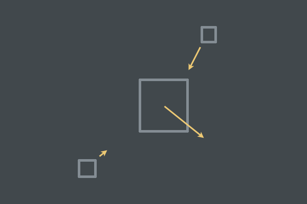
Lets take an example. Say we have a small circle representing a very heavy object. This small circle is flying around in the game, and it is so heavy that it pulls other objects towards it ever so slightly. Here is some rough pseudocode to demonstrate this:


HeavyObject object
for body in game do
  if(object.CloseEnoughTo( body )
    object.ApplyForcePullOn( body )

The function ApplyForcePullOn() could perhaps apply a small force to pull the body towards the HeavyObject, only if the body is close enough.

Two objects pulled towards a larger one. The pull force is dependent upon distance. — Two objects pulled towards a larger one moving pasted them. The pull forces are dependent upon their distance to the larger box.

It doesn't matter how many forces are added to the force of a body, as they will all add up to a single summed force vector for that body. This means that two forces acting upon the same body can potentially cancel each other out.

Broad Phase

In the previous article in this series collision detection routines were introduced. These routines were actually apart of what is known as the "narrow phase". The differences between broad phase and narrow phase can be researched rather easily with a Google search.

(In brief: we use broad phase collision detection to figure out which pairs of objects might be colliding, and then narrow phase collision detection to check whether they actually are colliding.)

I would like to provide some example code along with an explanation of how to implement a broad phase of \(O(n^2)\) time-complexity pair calculations.

\(O(n^2)\) essentially means that the time taken to check every pair of potential collisions will depend on the square of the number of objects. It uses Big-O notation.

Since we're working with pairs of objects, it will be useful to create a structure like so:


struct Pair
{
  body *A;
  body *B;
};

A broad phase should collect a bunch of possible collisions and store them all in Pair structures. These pairs can then be passed on to another portion of the engine (the narrow phase), and then resolved.

Example broad phase:


// Generates the pair list.
// All previous pairs are cleared when this function is called.
void BroadPhase::GeneratePairs( void )
{
  pairs.clear( )

  // Cache space for AABBs to be used in computation
  // of each shape's bounding box
  AABB A_aabb
  AABB B_aabb

  for(i = bodies.begin( ); i != bodies.end( ); i = i->next)
  {
    for(j = bodies.begin( ); j != bodies.end( ); j = j->next)
    {
      Body *A = &i->GetData( )
      Body *B = &j->GetData( )

      // Skip check with self
      if(A == B)
        continue

      A->ComputeAABB( &A_aabb )
      B->ComputeAABB( &B_aabb )

      if(AABBtoAABB( A_aabb, B_aabb ))
        pairs.push_back( A, B )
    }
  }
}

The above code is quite simple: Check each body against each body, and skip self-checks.

Culling Duplicates

There is one problem from the last section: many duplicate pairs will be returned! These duplicates need to be culled from the results. Some familiarity with sorting algorithms will be required here if you do not have some sort of sorting library available. If you're using C++ then you're in luck:


// Sort pairs to expose duplicates
sort( pairs, pairs.end( ), SortPairs );

// Queue manifolds for solving
{
  int i = 0;
  while(i < pairs.size( ))
  {
    Pair *pair = pairs.begin( ) + i;
    uniquePairs.push_front( pair );

    ++i;

    // Skip duplicate pairs by iterating i until we find a unique pair
    while(i < pairs.size( ))
    {
      Pair *potential_dup = pairs + i;
      if(pair->A != potential_dup->B || pair->B != potential_dup->A)
        break;
      ++i;
    }
  }
}

After sorting all the pairs in a specific order it can be assumed that all pairs in the pairs container will have all duplicates adjacent to one another. Place all unique pairs into a new container called uniquePairs, and the job of culling duplicates is finished.

The last thing to mention is the predicate SortPairs(). This SortPairs() function is what's actually used to do the sorting, and it might look like this:


bool SortPairs( Pair lhs, Pair rhs )
{
  if(lhs.A < rhs.A)
    return true;

  if(lhs.A == rhs.A)
    return lhs.B < rhs.B;

  return false;
}

The terms lhs and rhs can be read as "left hand side" and "right hand side". These terms are commonly used to refer to parameters of functions where things can logically be viewed as the left and right side of some equation or algorithm.

Layering

Layering refers to the act of having different objects never collide with one another. This is key for having bullets fired from certain objects not affect certain other objects. For example, players on one team might want their rockets to harm the enemies but not each other.

Layering is best implemented with bitmasks - see A Quick Bitmask How-To for Programmers and the Wikipedia page for a quick introduction, and the Filtering section of the Box2D manual to see how that engine uses bitmasks.

Layering should be done within the broad phase. Here I'll just paste a finished broad phase example:


// Generates the pair list.
// All previous pairs are cleared when this function is called.
void BroadPhase::GeneratePairs( void )
{
  pairs.clear( )

  // Cache space for AABBs to be used in computation
  // of each shape's bounding box
  AABB A_aabb
  AABB B_aabb

  for(i = bodies.begin( ); i != bodies.end( ); i = i->next)
  {
    for(j = bodies.begin( ); j != bodies.end( ); j = j->next)
    {
      Body *A = &i->GetData( )
      Body *B = &j->GetData( )

      // Skip check with self
      if(A == B)
        continue

      // Only matching layers will be considered
      if(!(A->layers & B->layers))
        continue;

      A->ComputeAABB( &A_aabb )
      B->ComputeAABB( &B_aabb )

      if(AABBtoAABB( A_aabb, B_aabb ))
        pairs.push_back( A, B )
    }
  }
}

Layering turns out to be both highly efficient and very simple.

Halfspace Intersection

A halfspace can be viewed as one side of a line in 2D. Detecting whether a point is on one side of a line or the other is a pretty common task, and should be understood thoroughly by anyone creating their own physics engine. It is too bad that this topic isn't really covered anywhere on the internet in a meaningful way, at least from what I've seen - until now, of course!

The general equation of a line in 2D is:

\[Equation 4:\\
General \: form: ax + by + c = 0\\
Normal \: to \: line: \begin{bmatrix}
a \\
b \\
\end{bmatrix}\]

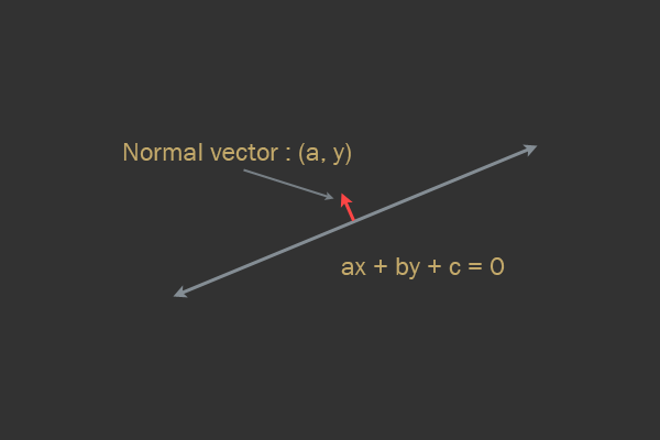
Note that, despite its name, the normal vector is not necessarily normalized (that is, it doesn't necessarily have a length of 1).

To see whether a point is on a particular side of this line, all that we need to do is plug the point into the x and y variables in the equation and check the sign of the result. A result of 0 means the point is on the line, and positive/negative mean different sides of the line.

That is all there is to it! Knowing this the distance from a point to the line is actually the result from the previous test. If the normal vector is not normalized, then the result will be scaled by the magnitude of the normal vector.

Conclusion

By now a complete, albeit simple, physics engine can be constructed entirely from scratch. More advanced topics such as friction, orientation, and dynamic AABB tree may be covered in future tutorials. Please ask questions or provide comments below, I enjoy reading and answering them!