Building a Financial Model with Pandas
Posted by Chris Moffitt in articles
Introduction
In my previous articles, I have discussed how to use pandas as a replacement for Excel as a data wrangling tool. In many cases, a python + pandas solution is superior to the highly manual processes many people use for manipulating data in Excel. However, Excel is used for many scenarios in a business environment - not just data wrangling. This specific post will discuss how to do financial modeling in pandas instead of Excel. For this example, I will build a simple amortization table in pandas and show how to model various outcomes.
In some ways, building the model is easier in Excel (there are many examples just a google search away). However, as an exercise in learning about pandas, it is useful because it forces one to think about how to use pandas strengths to solve a problem in a way different from the Excel solution. In my opinion the solution is more powerful because you can build on it to run multiple scenarios, easily chart various outcomes and focus on aggregating the data in a way most useful for your needs.
What is an amortization schedule?
Financial modeling can take many forms but for this article, I wanted to focus on a problem that many people will encounter in their lifetime. Namely, the finance aspects of a large loan.
The wikipedia page has a good explanation of an amortization schedule. In the simplest terms, an amortization schedule is a table that shows the periodic principal and interest payments needed to pay of a debt. The most common case is the payoff schedule for a mortgage.
Using the mortgage as an example, in each period (typically monthly) a home owner writes a check to their bank for a specified amount. This amount is split into a principal and interest payment. The bank keeps the interest and the principal is applied to the outstanding loan. Over a period of time the final balance will go to 0 and you will own the home.
Even with historically low interest rates, the amount of interest paid on a typical 15 or 30 year mortgage is very high. It is possible that you can pay almost as much in interest as the original loan was worth. Because of the financial importance of this purchase, it is important to understand all the financial ramifications of a mortgage. In addition, there are many variables that can affect the mortgage payments:
- Interest rate
- Duration of the loan
- Payment frequency (monthly vs bi-weekly, etc)
- Additional principal payments
There are certainly many on-line calculators and examples that show how to build tools in Excel. However, using the pandas solution is handy as a teaching tool to understand pandas in more detail and in using pandas to build a simple way to model and compare multiple scenarios. Before I go through the pandas-based solution, it’s helpful to see the Excel based solution so we have a model to use as a basis for the pandas solution:
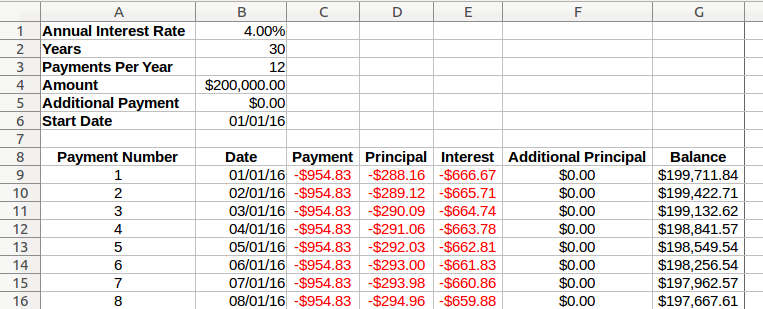
The basic model is simple. Each period results in a small decrease in the principal. At the end of 30 years, the balance is $0 and the loan is complete.
This model assumes that an individual pays exactly the prescribed amount each period. However, there can be financial benefits to paying extra principal and paying off the loan faster. As I think about modeling my mortgage, I’m curious to understand things like:
- How much do I save in interest if I contribute a little more principal each payment period?
- When will I pay off the loan?
- What is the impact of various interest rates?
Using the pandas solution can be useful for comparing and contrasting multiple options.
Payment, Principal and Interest
Not surprisingly, the numpy library has all the built in functions we need to do the behind the scenes math. In fact, the documentation shows one approach to build the amortization table. This approach certainly works but I’d like to include the results in a pandas DataFrame so that I can more easily dump the results to Excel or visualize the results.
I am going to walk through the basic parts of the solution for a 30 year $200K mortgage structured with a monthly payment and an annual interest rate of 4%. For an added twist, I’m going to build the solution with an extra $50/month to pay down the principal more quickly.
Get started with the imports of all the modules we need:
import pandas as pd
import numpy as np
from datetime import date
Define the variables for the mortgage:
Interest_Rate = 0.04
Years = 30
Payments_Year = 12
Principal = 200000
Addl_Princ = 50
start_date = (date(2016,1,1))
Now, let’s play with the basic formulas so we understand how they work.
Calculating the total payment requires us to pass the right values to the numpy
pmt
function.
pmt = np.pmt(Interest_Rate/Payments_Year, Years*Payments_Year, Principal)
-954.83059093090765
This means that every month we need to pay $954.83 (which matches the Excel solution above). But, how much of this is interest and how much is principal? Well, it depends. The payment stays constant over time but the amount applied to principal increases and the interest decreases as we move forward in time.
For example, for period 1, here is the interest and principal:
# Period to calculate
per = 1

# Calculate the interest
ipmt = np.ipmt(Interest_Rate/Payments_Year, per, Years*Payments_Year, Principal)

# Calculate the principal
ppmt = np.ppmt(Interest_Rate/Payments_Year, per, Years*Payments_Year, Principal)

print(ipmt, ppmt)
-666.6666666666667 -288.163924264
In other words, the first payment of $954.83 is composed of $666.67 in interest and only $288.16 in principal. Ouch.
Let’s look at what the breakdown is for period 240 (20 years in the future).
per = 240 # Period to calculate
# Calculate the interest
ipmt = np.ipmt(Interest_Rate/Payments_Year, per, Years*Payments_Year, Principal)

# Calculate the principal
ppmt = np.ppmt(Interest_Rate/Payments_Year, per, Years*Payments_Year, Principal)
print(ipmt, ppmt)
-316.49041533656924 -638.340175594
In this case, we are paying much more towards the principal ($638.34) and much less towards the interest ($316.49).
That should be fairly straightforward. But, what if I want to know what my balance is at period 240? Well, then I need to understand the cumulative effect of all my principal payments. This is not as straightforward in pandas. This is where the Excel solution is a little simpler to conceptualize.
In Excel, it is easy to reference the row above and use that value in the current row. Here is the Excel version for maintaining the balance due:

As you can see, in row 10, the balance formula references row 9. This type of formula is simple in Excel but in pandas a reference like this seems difficult. Your first instinct might be to try writing a loop but we know that is not optimal. Fortunately there is another approach that is more consistent with pandas. I will get to that in a moment. Before we go there, let’s get the basic pandas structure in place.
Building the Table
To answer the question about the balance change over time, we need to build a pandas DataFrame from scratch. There are extra steps here (as compared to Excel) but this is a useful adventure into some of the pandas functions I have not discussed previously.
First, let’s build a
DateTimeIndex
for the next 30 years based on
MS
(Month Start):
rng = pd.date_range(start_date, periods=Years * Payments_Year, freq='MS')
rng.name = "Payment_Date"
DatetimeIndex(['2016-01-01', '2016-02-01', '2016-03-01', '2016-04-01',
               '2016-05-01', '2016-06-01', '2016-07-01', '2016-08-01',
               '2016-09-01', '2016-10-01',
               ...
               '2045-03-01', '2045-04-01', '2045-05-01', '2045-06-01',
               '2045-07-01', '2045-08-01', '2045-09-01', '2045-10-01',
               '2045-11-01', '2045-12-01'],
              dtype='datetime64[ns]', name='Payment_Date', length=360, freq='MS')
This helpful function creates a range for the next 30 years starting on Jan 1, 2016.
The range will be used to build up the basic DataFrame we will use for the amortization schedule.
Note that we need to make sure the first period is 1 not 0, hence the need to use the
df.index += 1
:
df = pd.DataFrame(index=rng,columns=['Payment', 'Principal', 'Interest', 'Addl_Principal', 'Balance'], dtype='float')
df.reset_index(inplace=True)
df.index += 1
df.index.name = "Period"
Here is what the stub DataFrame looks like:
| Payment_Date | Payment | Principal | Interest | Addl_Principal | Balance | |
|---|---|---|---|---|---|---|
| Period | ||||||
| 1 | 2016-01-01 | NaN | NaN | NaN | NaN | NaN |
| 2 | 2016-02-01 | NaN | NaN | NaN | NaN | NaN |
| 3 | 2016-03-01 | NaN | NaN | NaN | NaN | NaN |
| 4 | 2016-04-01 | NaN | NaN | NaN | NaN | NaN |
| 5 | 2016-05-01 | NaN | NaN | NaN | NaN | NaN |
This looks similar to what we have in Excel so we’re on the right track.
Adding the payment is easy because it is a simple formula that produces a consistent value.
df["Payment"] = np.pmt(Interest_Rate/Payments_Year, Years*Payments_Year, Principal)
However the interest and principal change over time. Fortunately the formula is based on
the period which we have available in our DataFrame as
df.index
. We can
reference it in our formula to get the unique values for the specified period:
df["Principal"] = np.ppmt(Interest_Rate/Payments_Year, df.index, Years*Payments_Year, Principal)
df["Interest"] = np.ipmt(Interest_Rate/Payments_Year, df.index, Years*Payments_Year, Principal)
The final step is to add the Additional Principal (as a negative number) and round the values:
# Convert to a negative value in order to keep the signs the same
df["Addl_Principal"] = -Addl_Principal
df = df.round(2)
The table is starting to come together:
| Payment_Date | Payment | Principal | Interest | Addl_Principal | Curr_Balance | |
|---|---|---|---|---|---|---|
| Period | ||||||
| 1 | 2016-01-01 | -954.83 | -288.16 | -666.67 | -50 | NaN |
| 2 | 2016-02-01 | -954.83 | -289.12 | -665.71 | -50 | NaN |
| 3 | 2016-03-01 | -954.83 | -290.09 | -664.74 | -50 | NaN |
| 4 | 2016-04-01 | -954.83 | -291.06 | -663.78 | -50 | NaN |
| 5 | 2016-05-01 | -954.83 | -292.03 | -662.81 | -50 | NaN |
All that’s left is figuring out how to manage the
Curr_Balance
column.
Before I show you the better solution (I won’t say best because I would not
be surprised if there is an even better option), I am going to show you the
ugly approach I first took.
Maintaining the Balance - Try 1
I am showing this example because I suspect many novice pandas users would go down this path when trying to solve a similar problem. It also shows how a little time spent thinking about the solution yields a much better approach than just charging in with the first idea that comes to mind.
First, we calculate the balance for the first period by doing the calculation for the first row:
df["Balance"] = 0
df.loc[1, "Balance"] = Principal + df.loc[1, "Principal"] + df.loc[1, "Addl_Principal"]
| Payment_Date | Payment | Principal | Interest | Addl_Principal | Balance | |
|---|---|---|---|---|---|---|
| Period | ||||||
| 1 | 2016-01-01 | -954.830591 | -288.163924 | -666.666667 | -50 | 199661.836076 |
| 2 | 2016-02-01 | -954.830591 | -289.124471 | -665.706120 | -50 | 0.000000 |
| 3 | 2016-03-01 | -954.830591 | -290.088219 | -664.742372 | -50 | 0.000000 |
| 4 | 2016-04-01 | -954.830591 | -291.055180 | -663.775411 | -50 | 0.000000 |
| 5 | 2016-05-01 | -954.830591 | -292.025364 | -662.805227 | -50 | 0.000000 |
It works but it’s starting to get a little cumbersome.
My next step was to loop through each row and calculate the balance:
for i in range(2, len(df)+1):
    # Get the previous balance as well as current payments
    prev_balance = df.loc[i-1, 'Balance']
    principal = df.loc[i, 'Principal']
    addl_principal = df.loc[i, "Addl_Principal"]

    # If there is no balance, then do 0 out the principal and interest
    if prev_balance == 0:
        df.loc[i, ['Payment', 'Principal', 'Interest', 'Balance', 'Addl_Principal']] = 0
        continue

    # If this payment does not pay it off, reduce the balance
    if abs(principal + addl_principal) <= prev_balance:
        df.loc[i, 'Balance'] = principal + prev_balance + addl_principal

    # If it does pay it off, zero out the balance and adjust the final payment
    else:
        # Just adjust the principal down
        if prev_balance <= abs(principal):
            principal = -prev_balance
            addl_principal = 0
        else:
            addl_principal = (prev_balance - abs(principal_payment))
        df.loc[i, 'Balance'] = 0
        df.loc[i, 'Principal'] = principal
        df.loc[i, 'Addl_Principal'] = addl_principal
        df.loc[i, "Payment"] = principal +  df.loc[i, "Interest"]

df = df.round(2)
| Payment_Date | Payment | Principal | Interest | Addl_Principal | Balance | |
|---|---|---|---|---|---|---|
| Period | ||||||
| 1 | 2016-01-01 | -954.83 | -288.16 | -666.67 | -50 | 199661.84 |
| 2 | 2016-02-01 | -954.83 | -289.12 | -665.71 | -50 | 199322.71 |
| 3 | 2016-03-01 | -954.83 | -290.09 | -664.74 | -50 | 198982.62 |
| 4 | 2016-04-01 | -954.83 | -291.06 | -663.78 | -50 | 198641.57 |
| 5 | 2016-05-01 | -954.83 | -292.03 | -662.81 | -50 | 198299.54 |

Oh boy. That works but the code smell is quite intense. At this point, I almost ditched this article because the solution was not very pretty.
I decided to regroup by doing some research and found this post by Brandon Rhodes which helped me re-frame my problem and develop a much better solution.
Maintaining the Balance - Try 2
After reading Brandon’s article, I realized that by adding an additional column with my cumulative principal payments, I could very easily calculate the balance. The pandas authors realized some of the challenges of calculating results based on prior rows of data so they included several cumulative functions.
In this example, I will use
cumsum
to build a running total of my
principal payments.
df["Cumulative_Principal"] = (df["Principal"] + df["Addl_Principal"]).cumsum()
One thing that is interesting is that with the additional principal payments, I end up with paying more in principal that I originally planned to.
| Payment_Date | Payment | Principal | Interest | Addl_Principal | Curr_Balance | Cumulative_Principal | |
|---|---|---|---|---|---|---|---|
| Period | |||||||
| 356 | 2045-08-01 | -954.83 | -939.07 | -15.76 | -50 | NaN | -214012.32 |
| 357 | 2045-09-01 | -954.83 | -942.20 | -12.63 | -50 | NaN | -215004.52 |
| 358 | 2045-10-01 | -954.83 | -945.35 | -9.49 | -50 | NaN | -215999.87 |
| 359 | 2045-11-01 | -954.83 | -948.50 | -6.33 | -50 | NaN | -216998.37 |
| 360 | 2045-12-01 | -954.83 | -951.66 | -3.17 | -50 | NaN | -218000.03 |
This is obviously not correct so I need to put a floor (or
clip
) the results
so that I never exceed $200,000 in total principal payments:
df["Cumulative_Principal"] = df["Cumulative_Principal"].clip(lower=-Principal)
Now that I have that out of the way, the Current Balance for any given period is very simple to calculate:
df["Curr_Balance"] = Principal + df["Cumulative_Principal"]
| Payment_Date | Payment | Principal | Interest | Addl_Principal | Curr_Balance | Cumulative_Principal | |
|---|---|---|---|---|---|---|---|
| Period | |||||||
| 1 | 2016-01-01 | -954.83 | -288.16 | -666.67 | -50 | 199661.84 | -338.16 |
| 2 | 2016-02-01 | -954.83 | -289.12 | -665.71 | -50 | 199322.72 | -677.28 |
| 3 | 2016-03-01 | -954.83 | -290.09 | -664.74 | -50 | 198982.63 | -1017.37 |
| 4 | 2016-04-01 | -954.83 | -291.06 | -663.78 | -50 | 198641.57 | -1358.43 |
| 5 | 2016-05-01 | -954.83 | -292.03 | -662.81 | -50 | 198299.54 | -1700.46 |
Wow. This approach is much simpler than the looping solution I tried in my first iteration. The only thing left is figuring out how to clean up the table if we pay it off early.
The Big Payoff
When an amortization table is built, the assumption is that the payments over each period will just be enough to cover the principal and interest and at the end of the time period, the balance goes to 0. However, there may be scenarios where you want to accelerate the payments in order to pay off the loan earlier. In the example we have been running with, the model includes $50 extra each month.
In order to find the last payment, we want to find the the payment where the Curr_Balance first goes to 0:
| Payment_Date | Payment | Principal | Interest | Addl_Principal | Curr_Balance | Cumulative_Principal | |
|---|---|---|---|---|---|---|---|
| Period | |||||||
| 340 | 2044-04-01 | -954.83 | -890.38 | -64.45 | -50 | 1444.24 | -198555.76 |
| 341 | 2044-05-01 | -954.83 | -893.35 | -61.48 | -50 | 500.89 | -199499.11 |
| 342 | 2044-06-01 | -954.83 | -896.33 | -58.50 | -50 | 0.00 | -200000.00 |
| 343 | 2044-07-01 | -954.83 | -899.32 | -55.52 | -50 | 0.00 | -200000.00 |
Based on this view, you can see that our last payment would be in period 342.
We can find this value by using
idxmax
last_payment = df.query("Curr_Balance <= 0")["Curr_Balance"].idxmax(axis=1, skipna=True)
df.loc[last_payment]
Payment_Date            2044-06-01 00:00:00
Payment                             -954.83
Principal                           -896.33
Interest                              -58.5
Addl_Principal                          -50
Curr_Balance                              0
Cumulative_Principal                -200000
Name: 342, dtype: object
Now we know the last payment period, but astute readers may have noticed
that we payed $896.33 + $50 in principal but we only owed $500.89. We can clean
this up with a couple of statements using
last_payment
as the index:
df.loc[last_payment, "Principal"] = -(df.loc[last_payment-1, "Curr_Balance"])
df.loc[last_payment, "Payment"] = df.loc[last_payment, ["Principal", "Interest"]].sum()
df.loc[last_payment, "Addl_Principal"] = 0
| Payment_Date | Payment | Principal | Interest | Addl_Principal | Curr_Balance | Cumulative_Principal | |
|---|---|---|---|---|---|---|---|
| Period | |||||||
| 338 | 2044-02-01 | -954.83 | -884.48 | -70.36 | -50 | 3322.04 | -196677.96 |
| 339 | 2044-03-01 | -954.83 | -887.42 | -67.41 | -50 | 2384.62 | -197615.38 |
| 340 | 2044-04-01 | -954.83 | -890.38 | -64.45 | -50 | 1444.24 | -198555.76 |
| 341 | 2044-05-01 | -954.83 | -893.35 | -61.48 | -50 | 500.89 | -199499.11 |
| 342 | 2044-06-01 | -559.39 | -500.89 | -58.50 | 0 | 0.00 | -200000.00 |
For a final step, we can truncate the DataFrame so that we only include through period 342:
df = df.loc[0:last_payment]
Now we have a complete table, we can summarize and compare results.
Time to Analyze
It has taken some time to pull this solution together but now that we know how to solve the problem, we can put it into a function that allows us to input various scenarios, summarize the results and visualize them in various ways.
I have built an amortization table function that looks like this:
def amortization_table(interest_rate, years, payments_year, principal, addl_principal=0, start_date=date.today()):
    """ Calculate the amortization schedule given the loan details

     Args:
        interest_rate: The annual interest rate for this loan
        years: Number of years for the loan
        payments_year: Number of payments in a year
        principal: Amount borrowed
        addl_principal (optional): Additional payments to be made each period. Assume 0 if nothing provided.
                                   must be a value less then 0, the function will convert a positive value to
                                   negative
        start_date (optional): Start date. Will start on first of next month if none provided

    Returns:
        schedule: Amortization schedule as a pandas dataframe
        summary: Pandas dataframe that summarizes the payoff information
    """
Refer to this notebook for the full code as well as example usage.
You can call it to get summary info as well as the detailed amortization schedule:
schedule1, stats1 = amortization_table(0.05, 30, 12, 100000, addl_principal=0)
Which yields a schedule:
| Payment_Date | Payment | Principal | Interest | Addl_Principal | Curr_Balance | Cumulative_Principal | |
|---|---|---|---|---|---|---|---|
| Period | |||||||
| 1 | 2016-12-01 | -536.82 | -120.15 | -416.67 | 0 | 99879.85 | -120.15 |
| 2 | 2017-01-01 | -536.82 | -120.66 | -416.17 | 0 | 99759.19 | -240.81 |
| 3 | 2017-02-01 | -536.82 | -121.16 | -415.66 | 0 | 99638.03 | -361.97 |
| 4 | 2017-03-01 | -536.82 | -121.66 | -415.16 | 0 | 99516.37 | -483.63 |
| 5 | 2017-04-01 | -536.82 | -122.17 | -414.65 | 0 | 99394.20 | -605.80 |
and summary stats:
| payoff_date | Interest Rate | Number of years | Period_Payment | Payment | Principal | Addl_Principal | Interest | |
|---|---|---|---|---|---|---|---|---|
| 0 | 11-01-2046 | 0.05 | 30 | -536.82 | -193255.2 | -100000.02 | 0.0 | -93255.69 |
The powerful aspect of this approach is that you can run multiple scenarios and combine them into 1 table:
schedule2, stats2 = amortization_table(0.05, 30, 12, 100000, addl_principal=-200)
schedule3, stats3 = amortization_table(0.04, 15, 12, 100000, addl_principal=0)

# Combine all the scenarios into 1 view
pd.concat([stats1, stats2, stats3], ignore_index=True)
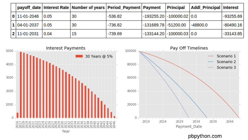
| payoff_date | Interest Rate | Number of years | Period_Payment | Payment | Principal | Addl_Principal | Interest | |
|---|---|---|---|---|---|---|---|---|
| 0 | 11-01-2046 | 0.06 | 30 | -599.55 | -215838.00 | -99999.92 | 0.0 | -115838.23 |
| 1 | 04-01-2037 | 0.05 | 30 | -736.82 | -131689.78 | -51200.00 | -48800.0 | -80490.16 |
| 2 | 11-01-2031 | 0.04 | 15 | -739.69 | -133144.20 | -100000.03 | 0.0 | -33143.85 |
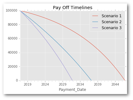
Finally, because the data is in a DataFrame, we can easily plot the results to see what the payoff time lines look like for the various scenarios:
fig, ax = plt.subplots(1, 1)
schedule1.plot(x='Payment_Date', y='Curr_Balance', label="Scenario 1", ax=ax)
schedule2.plot(x='Payment_Date', y='Curr_Balance', label="Scenario 2", ax=ax)
schedule3.plot(x='Payment_Date', y='Curr_Balance', label="Scenario 3", ax=ax)
plt.title("Pay Off Timelines")
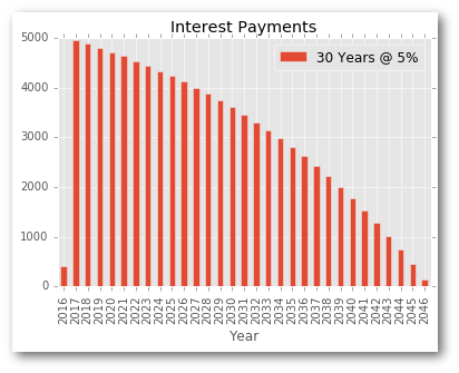
Or, we can look at the interest payments by year:
fig, ax = plt.subplots(1, 1)

y1_schedule = schedule1.set_index('Payment_Date').resample("A")["Interest"].sum().abs().reset_index()
y1_schedule["Year"] = y1_schedule["Payment_Date"].dt.year
y1_schedule.plot(kind="bar", x="Year", y="Interest", ax=ax, label="30 Years @ 5%")

plt.title("Interest Payments");
Obviously there are lots of available options for visualizing the results but this gives you a flavor for some of the options.
Closing Out
Thank you for reading through this example. I have to admit that this was one of my more time consuming articles. It was also one where I learned a lot about how to work with pandas and use some functions that I did not have much familiarity with. I hope this article will help others build their knowledge of python and pandas and might even be useful as a tool to analyze your own mortgage payment options.
Article Updates
Nov-26-2016 - Calculation Accuracy:
Based on feedback in the comments and discussions off-line, I realized that the calculations are not correctly working with the extra principal payments. After looking into this in more detail, I figured out that the interest and principal payments do indeed to be recalculated each period which is proving to be problematic in pandas. I am working on a solution but in the meantime want to make sure to note the issue.
I am keeping the article up since I think it is helpful to show additional pandas functionality but do regret that the results are not correct.
If you have ideas on how to fix, please let me know.
Dec-19-2016 - Corrected Article:
- A new article has been posted that contains corrected code to fix the errors identified above.
Dec-13-2019 - Removed
ix
- Removed
ixand usedlocto be compatible with current version of pandas. - Also updated the referenced notebook with the
.locusage
Comments